Envariance and the Origin of Probabilities in Quantum Mechanics¶

This week I'd like to talk about some of Wojciech Zurek's ideas in the foundations of quantum mechanics.

But first, a word of caution. Philosophically speaking, any time you try to prove something you have to choose a starting place, and the question is whether you can get from A to B. We're going to try to demonstrate how probabilities arise in quantum mechanics, but we're not going to start from scratch: we're going to assume all of unitary quantum mechanics, with its Hilbert spaces, tensor products, entanglements, and so forth. Indeed, Zurek's whole endeavor is to derive Born's rule for probabilities from a consideration of the nature of entanglement. In some sense, this could be seen as merely shuffling pieces around the board, substituting one mysterious things for another: e.g., we're not going to explain "why entanglement", but instead "why probabilities given entanglement."

At the same time, there is some justification for this approach. After all, consider the lonely, isolated qubit in a pure state. There is, I think, a very real question about what exactly is "quantum" about it at all. A classical spinning object can be defined in terms of its oriented axis of rotation, and the phase of its rotation around that axis: in other words, a point on a sphere, and a point on a circle. And this is exactly, no more and no less, the information encoded in the qubit's state vector.

We recall: given the state of a qubit quantized along the $Z$ axis, $\mid \phi \rangle = \begin{pmatrix} \alpha \\ \beta \end{pmatrix}$, we can interpret its two complex components as picking out a point on the sphere via $(\langle \phi \mid X \mid \phi \rangle, \langle \phi \mid Y \mid \phi \rangle, \langle \phi \mid Z \mid \phi \rangle)$, or more directly in terms of the complex ratio $\frac{\beta}{\alpha}$, which, stereographically projected from the complex plane to the unit sphere, gives the point on the sphere. (If $\alpha = 0$, we get end up at the South Pole, the point of projection).

So in some sense, we're just working with a somewhat unfamiliar complex representation of a point on a sphere plus phase: the ratio between the two components specifies a point on the sphere up to multiplication by a complex number, the latter of which must be a phase (if we've demanded normalization $\mid \alpha \mid^2 + \mid \beta \mid^2 = 1$) which can represent the phase of the rotation around the given axis. (That we're working with a half integer representation of $SU(2)$ is not wholly relevant to the point here.)

Normally, we'd describe a point on the sphere in terms of cartesian coordinates as a "superposition" of basis states: $(1,0,0), (0,1,0), (0,0,1)$, each of which are orthogonal in "real space". In our complex representation, it happens that qubit states which are orthogonal complex vectors correspond to antipodal or opposite points on the sphere. So that we can describe a point on the sphere as a complex linear superposition of the vectors corresponding to any two opposite points on the sphere. Above, we chose the two points along the $Z$ axis, but any would do.

So what's quantum about our qubit? The quantum part comes into play only when we consider how the qubit interacts with the world: when it is measured and when it gets entangled: and in some sense, these are the same thing from different perspectives.

The original logical positivist genius of quantum mechanics was to describe systems as being in linear combinations of states corresponding to outcomes to experiments: these orthogonal states can all be encoded as the eigenvectors of some Hermitian operator, whose real eigenvalues correspond to the measured numerical values associated to outcomes (what had been, classically, position, momentum, etc.) The relevant experiment for the qubit is the Stern-Gerlach apparatus: send a spin-$\frac{1}{2}$ through the magnetic field and it ends up either taking the high road or the low road; and if it takes the high road, it's in the $\mid \uparrow \rangle$ state relative to the Stern-Gerlach axis; and if it takes the down road, it's in the $\mid \downarrow \rangle$ state. So these are the two outcomes: the two outcomes correspond to opposite points on the sphere. Each occurs with a certain probability. How do we get the probability? We describe the state of the qubit as a complex linear superposition $\alpha \mid \uparrow \rangle + \beta \mid \downarrow \rangle$, where $\uparrow$ and $\downarrow$ are along the axis of the magnetic field, and then the probabilities are given by the norm squared of the amplitudes, $Pr(\uparrow) = \mid \alpha \mid^2$ and $Pr(\downarrow) = \mid \beta \mid^2$. This is Born's rule.

So what we approached first in purely geometrical terms now has this extra probabalistic overlay: what makes the qubit quantum is precisely how it behaves when we interact with it.

But we could take a third person perspective on the measurement interaction and describe it in terms of entanglement. After all, in the Stern-Gerlach experiment, we don't measure the qubit directly: we measure its position, which becomes entangled with the spin in the course of the unitary evolution instigated by the set-up.

$$\alpha \mid \uparrow \rangle + \beta \mid \downarrow \rangle \Rightarrow \alpha \mid \uparrow \Uparrow \rangle + \beta \mid \downarrow \Downarrow \rangle$$

Operationally, if we measure the position, we get $\mid \Uparrow \rangle$ or $\mid \Downarrow \rangle$ with the same probabilities as before. Whatever answer we get, the qubit state will be perfectly correlated with the position state. This, after all, is what we mean by an accurate measurement.

But of course, we don't really measure the position directly either, but some proxy of it, so that, including all of various apparatuses in the picture, including in principle the photons by which the experimenter observes the outcome on the dial, even the neurons in the experimenter's brain that fire or don't fire depending on the outcome, we end up with a chain of entanglement:

$$\alpha \mid \uparrow \rangle + \beta \mid \downarrow \rangle \Rightarrow \alpha \mid \uparrow \Uparrow \upharpoonright \dots \rangle + \beta \mid \downarrow \Downarrow \downharpoonright \dots \rangle$$

And yet when the buck does stop, we get an answer at random. Why? By exploring the implications of entanglement, we're going to try to resolve this question about probability.

Recall the following image from our string diagram days:

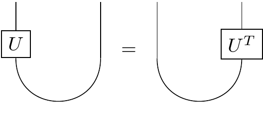
Here the wires could represent qubits. Then the $\cup$ would represent the maximally entangled state $\frac{1}{\sqrt{2}}(\mid \uparrow \uparrow \rangle + \mid \downarrow \downarrow \rangle)$, and the individual boxes would be $2 \times 2 $ linear operators. What this equation is saying is that a unitary operator acting on one half of the $\cup$ has exactly the same effect as acting on the other half with its transpose. Indeed, we can think of the operator sliding around the cup like a bead on a string, arriving "upside down" on the other side.

E.g.:

from spheres import *

def left(O):
    return qt.tensor(O, qt.identity(2))

def right(O):
    return qt.tensor(qt.identity(2), O)

cup = qt.bell_state("00")
U = qt.rand_unitary(2)

left(U)*cup

We've acted with a unitary on the left. It's just the same as acting on the right with its transpose:

right(U.trans())*cup

The defining feature of a unitary operator is that its inverse is given by its conjugate transpose: $UU^{\dagger} = I$. Now naturally, the conjugate transpose of the transpose of an operator is just the conjugate of the operator: $(U^{T})^{\dagger} = U^{*}$. So that:

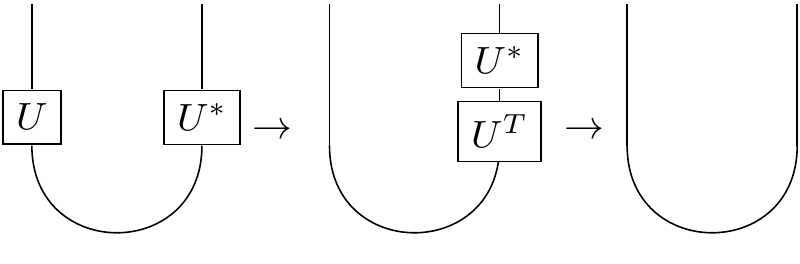
In other words, acting on the left with $U$ and on the right with $U^{*}$ amounts to doing nothing at all!

In other words, due to entanglement, there is a symmetry: if I act on the left with any $U$, you can always undo it by acting on the right with $U^{*}$. Zurek terms this symmetry resulting from entanglement "envariance" or "entanglement assisted invariance."

right(U.conj())*left(U)*cup

dirac(right(U.conj())*left(U)*cup)

0.707 |00> Pr: 0.500
0.707 |11> Pr: 0.500

Something analogous holds true for any maximally entangled state.

Recall that I can obtain any maximally entangled state by acting on the cup (on the left, say) with some unitary operator.

In other words, there's a duality between unitary operators and maximally entangled states:

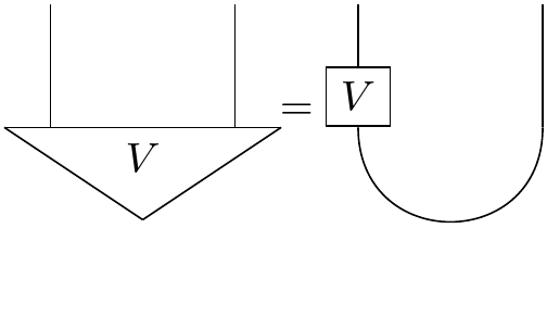
In fact, acting on the left of the $\cup$ with the operator $V$ amounts to "splaying out" the components of the matrix as a vector:

$$\begin{pmatrix} a & b \\ c & d \end{pmatrix} \rightarrow \frac{1}{\sqrt{2}}\begin{pmatrix}a \\ b \\ c \\ d \end{pmatrix}$$

V = qt.rand_unitary(2)
V

V_cup = left(V)*cup
np.sqrt(2)*V_cup

By looking at the Von Neumann entropy, we can confirm that the state $\mid V \rangle$ is itself a maximally entangled state: which stands to reason, since we started off with a maximally entangled state, and by acting unitarily on only a part, we can't change the amount of entanglement.

print(qt.entropy_vn(V_cup.ptrace(0)))
print(qt.entropy_vn(V_cup.ptrace(1)))
print(np.log(2)) # max entropy

0.6931471805599453
0.6931471805599453
0.6931471805599453

So suppose we act with $U$ on the left on some arbitrary maximally entangled state.

We could rewrite things like:

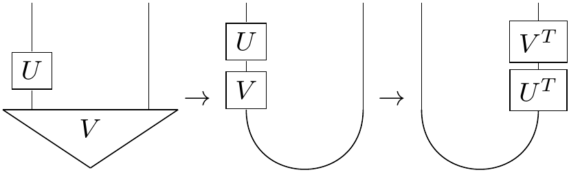
We could then consider acting on the right with $V^{T}U^{*}V^{*}$:

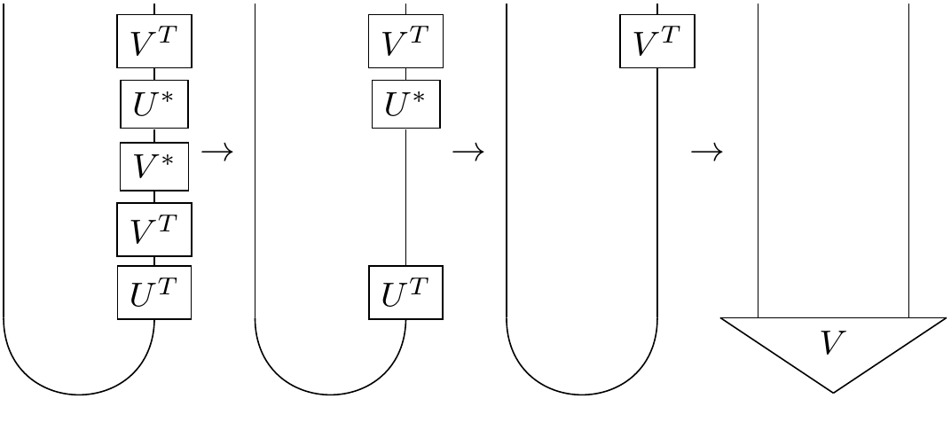
The $V^{*}$ cancels out the $V^{T}$, the $U^{*}$ cancels out the $U^{T}$, and then the $V^{T}$ restores the original maximally entangled state.

Thus:

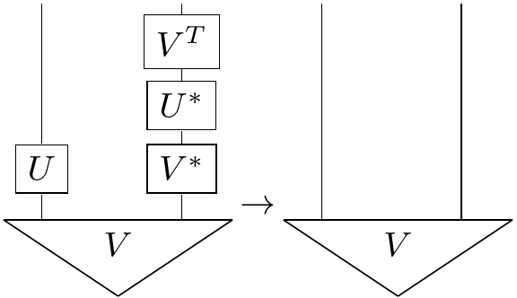
So given an maximally entangled state, we can always cancel out the action of some unitary $U$ on the left by a corrresponding unitary on the right.

V_cup

right(V.trans()*U.conj()*V.conj())*left(U)*V_cup

Vright = V.trans()*U.conj()*V.conj()
print("Is unitary? %s" % np.allclose(Vright*Vright.dag(), qt.identity(2)))

Is unitary? True

Another way of thinking about this is in terms of the Schmidt decomposition.

Given a bipartite state of two systems $A$ and $B$, which live in Hilbert spaces of dimensions $d_{A}$ and $d_{B}$ respectively, we can reshape its vector components into a $d_{A} \times d_{B}$ matrix, so that:

$$ \mid \psi \rangle_{AB} = \sum_{j=1}^{d_{A}} \sum_{k=1}^{d_{B}} C_{jk} \mid j \rangle_{A} \mid k \rangle_{B} $$

Here $\mid j \rangle$ and $\mid k \rangle$ refer to the standard basis.

We can then take the singular value decomposition of this matrix:

$$ C = Y \Sigma Z $$

Where $Y$ is a $d_{a} \times d_{a}$ unitary, $Z$ is a $d_{b} \times d_{b}$ unitary, and $\Sigma$ is a $d_{A} \times d_{B}$ diagonal matrix with the "singular values" (in decreasing order, by convention) along the diagonal: these singular values are real and non-negative.

We can then form new orthogonal basis sets for $A$ and $B$:

$$\mid i \rangle_{A} = \sum_{j} Y_{ji}\mid j \rangle_{A}$$$$\mid i \rangle_{B} = \sum_{k} Z_{ik}\mid k \rangle_{B}$$

If $\sigma_{i}$ is the vector of the singular values, then we can rewrite our state in the "Schmidt basis":

$$ \mid \psi \rangle_{AB} = \sum_{i=1}^{d_{A}} \sigma_{i} \mid i \rangle_{A} \mid i \rangle_{B} $$

So for example, taking a random two qubit state, let's reshape the components into a matrix:

state = qt.rand_ket(4)
state_matrix = components(state).reshape(2,2)
qt.Qobj(state_matrix)

And confirm the SVD works as promised:

Y, s, Z = np.linalg.svd(state_matrix)
qt.Qobj(Y @ np.diag(s) @ Z)

Then let's form the new orthogonal basis sets for $A$ and $B$, and check that we recover the original state:

A = [sum([Y[j,i]*qt.basis(2, j) for j in range(2)]) for i in range(2)]
B = [sum([Z[i,k]*qt.basis(2, k) for k in range(2)]) for i in range(2)]
schmidt = sum([s[i]*qt.tensor(A[i], B[i]) for i in range(2)])

schmidt

So given a bipartite state we can always rewrite it in the Schmidt basis as a sum over separable states in $A$ and $B$, such that the components in that basis are real valued and non-negative.

If we consider the Schmidt decomposition of a two qubit separable state, then naturally it will have only one singular value, which will be $1$: the state can be written as a simple outer product. Another way of saying this is that the matrix is rank-1: indeed, the rank of a matrix is given by the number of non-zero singular values.

separable = qt.tensor(qt.rand_ket(2), qt.rand_ket(2))
Y, s, Z = np.linalg.svd(components(separable).reshape(2,2))
s

array([1.00000000e+00, 2.91727029e-16])

Let's consider any old random state. Generically, it will be somewhat entangled, and have two different singular values.

any_old = qt.rand_ket(4)
any_old.dims = [[2,2],[1,1]]
Y, s, Z = np.linalg.svd(components(any_old).reshape(2,2))
print(s)

[0.91786817 0.39688539]

Finally, let's consider a maximally entangled state:

max_entangled = left(qt.rand_unitary(2))*cup
Y, s, Z = np.linalg.svd(components(max_entangled).reshape(2,2))
print(s)

[0.70710678 0.70710678]

It always has two singular values--and they're the same. This tells us what we already know, that any maximally entangled state is just the $\cup$ in disguise. In any dimension, a maximally entangled state always has a maximal Schmidt rank, and all its singular values are the same.

Following this nice paper, another way of calculating an operator that, when it acts on the right, cancels out the action of $U$ on the left, is as follows:

We express $U$ in the Schmidt basis via:

$$\tilde{U} = Y^{\dagger}UY$$

We can construct an operator:

$$\tilde{V} = (\Sigma_{R}^{-1}\tilde{U}\Sigma)^{T}$$

Since our state has maximal Schmidt rank, a right inverse of $\Sigma$, $\Sigma_{R}^{-1}$ such that $\Sigma\Sigma_{R}^{-1} = I_{d_{A}}$ will exist.

In the original basis, this would be:

$$V = Z^{T}\tilde{V}Z^{*}$$

Following out the algebra, we can write this more directly as:

$$V = (C_{R}^{-1}UC)^{T}$$

Where:

$$C_{R}^{-1} = Z^{\dagger}\Sigma_{R}^{-1}Y^{\dagger}$$

Then the action of $U$ on the left will be equivalent to the action of $V$ on the right:

$$ (U \otimes I)\mid \psi \rangle_{AB} = (I \otimes V)\mid \psi \rangle_{AB} $$

So:

$$ V_{B}^{\dagger}U_{A}\mid \psi \rangle_{AB} = \mid \psi \rangle_{AB} $$

Indeed, maximal entanglement is equivalent to there existing some such $U$ and $V$, which is the same as saying: the state has maximal rank and all the singular values are equal.

Fully (but not necessarily maximally) entangled states correspond to the case where the Schmidt rank is maximal. Then $\Sigma$ is invertible, and we have $U\Sigma = \Sigma V^{T}$, and the action of $U_{A}$ is equivalent to the action of $V_{B}$. But unless the state is maximally entangled, $V_{B}$ won't be unitary!

def schmidt_test(state, U):
    state.dims = [[2,2], [1,1]]
    print("the state:")
    dirac(state)
    dm0 = state.ptrace(0)
    print("\ndm of subsystem:")
    print(dm0)
    print("entropy of subsystem / max entropy: %.3f" % (qt.entropy_vn(dm0)/np.log(2)))

    C = components(state).reshape(2,2)
    Y, s, Z = np.linalg.svd(C)
    print("singular values: %s" % s)

    S = np.diag(s)
    S_inv = np.linalg.inv(S)
    C, Y, S, S_inv, Z = qt.Qobj(C), qt.Qobj(Y), qt.Qobj(S), qt.Qobj(S_inv), qt.Qobj(Z)

    U_tilde = Y.dag()*U*Y
    V_tilde = (S_inv*U_tilde*S).trans()
    V = Z.trans()*V_tilde*Z.conj()
    V2 = (Z.dag()*S_inv*Y.dag()*U*C).trans()
    
    print("\nU:\n%s\n" % U)
    print("V == V2? %s" % np.allclose(V, V2))
    print("V unitary? %s" % (np.allclose(V*V.dag(), np.eye(2))))
    print("U_L|psi> == V_R|psi>? %s" % np.allclose(left(U)*state, right(V)*state))
    print("Vdag_R*U_L|psi> == |psi>? %s" % np.allclose(right(V.dag())*left(U)*state, state))

Let's check it out for the $\cup$ state:

schmidt_test(qt.bell_state("00"), qt.rand_unitary(2))

the state:
0.707 |00> Pr: 0.500
0.707 |11> Pr: 0.500

dm of subsystem:
Quantum object: dims = [[2], [2]], shape = (2, 2), type = oper, isherm = True
Qobj data =
[[0.5 0. ]
 [0.  0.5]]
entropy of subsystem / max entropy: 1.000
singular values: [0.70710678 0.70710678]

U:
Quantum object: dims = [[2], [2]], shape = (2, 2), type = oper, isherm = False
Qobj data =
[[ 0.88488301+0.02399593j  0.32363549-0.33416513j]
 [-0.45755751-0.0839487j   0.70627098-0.53364317j]]

V == V2? True
V unitary? True
U_L|psi> == V_R|psi>? True
Vdag_R*U_L|psi> == |psi>? True

We can see it also works for a generic maximally entangled state:

schmidt_test(left(qt.rand_unitary(2))*qt.bell_state("00"), qt.rand_unitary(2))

the state:
0.628+0.325i |00> Pr: 0.500
0.605+0.367i |11> Pr: 0.500

dm of subsystem:
Quantum object: dims = [[2], [2]], shape = (2, 2), type = oper, isherm = True
Qobj data =
[[0.5 0. ]
 [0.  0.5]]
entropy of subsystem / max entropy: 1.000
singular values: [0.70710678 0.70710678]

U:
Quantum object: dims = [[2], [2]], shape = (2, 2), type = oper, isherm = False
Qobj data =
[[0.98818773+0.15324821j 0.        +0.j        ]
 [0.        +0.j         0.8414322 -0.5403627j ]]

V == V2? True
V unitary? True
U_L|psi> == V_R|psi>? True
Vdag_R*U_L|psi> == |psi>? True

What about for a separable state?

schmidt_test(qt.tensor(qt.rand_ket(2), qt.rand_ket(2)), qt.rand_unitary(2))

the state:
-0.036+-0.462i |00> Pr: 0.214
-0.010+-0.609i |01> Pr: 0.371
-0.375+0.104i |10> Pr: 0.152
-0.501+0.107i |11> Pr: 0.263

dm of subsystem:
Quantum object: dims = [[2], [2]], shape = (2, 2), type = oper, isherm = True
Qobj data =
[[ 0.58569255+0.j         -0.09445277+0.48346195j]
 [-0.09445277-0.48346195j  0.41430745+0.j        ]]
entropy of subsystem / max entropy: -0.000
singular values: [1.00000000e+00 7.50848834e-17]

U:
Quantum object: dims = [[2], [2]], shape = (2, 2), type = oper, isherm = False
Qobj data =
[[0.99902344+0.04418341j 0.        +0.j        ]
 [0.        +0.j         0.92136142+0.388707j  ]]

V == V2? True
V unitary? False
U_L|psi> == V_R|psi>? False
Vdag_R*U_L|psi> == |psi>? False

What about for some generic state?

schmidt_test(qt.rand_ket(4), qt.rand_unitary(2))

the state:
-0.212+-0.306i |00> Pr: 0.139
0.375+0.411i |01> Pr: 0.310
0.487+0.218i |10> Pr: 0.284
-0.433+-0.283i |11> Pr: 0.267

dm of subsystem:
Quantum object: dims = [[2], [2]], shape = (2, 2), type = oper, isherm = True
Qobj data =
[[ 0.4484237 +0.j         -0.44842718-0.17484892j]
 [-0.44842718+0.17484892j  0.5515763 +0.j        ]]
entropy of subsystem / max entropy: 0.118
singular values: [0.99200065 0.12623279]

U:
Quantum object: dims = [[2], [2]], shape = (2, 2), type = oper, isherm = False
Qobj data =
[[0.99962461+0.0273978j  0.        +0.j        ]
 [0.        +0.j         0.54696455-0.83715577j]]

V == V2? True
V unitary? False
U_L|psi> == V_R|psi>? True
Vdag_R*U_L|psi> == |psi>? False

We can see that for a generic non-maximally entangled state, $V$ might exist but it won't be unitary.

What about for a generic post-measurement state?

a, b = components(qt.rand_ket(2))
schmidt_test(a*bitstring_basis("00") + b*bitstring_basis("11"), qt.rand_unitary(2))

the state:
-0.694+0.237i |00> Pr: 0.537
-0.065+-0.677i |11> Pr: 0.463

dm of subsystem:
Quantum object: dims = [[2], [2]], shape = (2, 2), type = oper, isherm = True
Qobj data =
[[0.53736211 0.        ]
 [0.         0.46263789]]
entropy of subsystem / max entropy: 0.996
singular values: [0.73304987 0.68017489]

U:
Quantum object: dims = [[2], [2]], shape = (2, 2), type = oper, isherm = False
Qobj data =
[[ 0.79811267+0.02712935j -0.32878448+0.50416359j]
 [ 0.50046488+0.33438761j  0.72323488-0.33860173j]]

V == V2? True
V unitary? False
U_L|psi> == V_R|psi>? True
Vdag_R*U_L|psi> == |psi>? False

We can see that it works sometimes: specifically in the case where $U$ is diagonal. Indeed, in general, states may be envariant under certain unitaries--but maximally entangled states are envariant under all unitaries.

And incidentally, all the above generalizes to general bipartitions of multipartite systems. For $\mid \psi \rangle_{ABC}$, maximally entangled across $A$ and $BC$, any operator on $A$ is equivalent to some operator on $BC$ (but not necessarily the other way around).

Finally, in view of what we're about to discuss, let's consider the action of the $X$ operator, which can be written:

$$\mid \uparrow \rangle \langle \downarrow \mid + \mid \downarrow \rangle \langle \uparrow \mid$$

It's unitary and hermitian, which means that it's its own inverse.

Acting on a qubit, it swaps $\uparrow$ and $\downarrow$ in the $Z$ basis.

qubit = qt.rand_ket(2)

dirac(qubit)
print()
dirac(qt.sigmax()*qubit)

0.015+-0.708i |0> Pr: 0.501
0.642+-0.295i |1> Pr: 0.499

0.642+-0.295i |0> Pr: 0.499
0.015+-0.708i |1> Pr: 0.501

Acting on the $\cup$, $X$ flips the correlations: we get the anticorrelated state instead:

$$ X_{L} \frac{1}{\sqrt{2}}(\mid \uparrow \uparrow \rangle + \mid \downarrow \downarrow \rangle) \rightarrow \frac{1}{\sqrt{2}}(\mid \downarrow \uparrow \rangle + \mid \uparrow \downarrow \rangle)$$

dirac(cup)
print()
dirac(left(qt.sigmax())*cup)

0.707 |00> Pr: 0.500
0.707 |11> Pr: 0.500

0.707 |01> Pr: 0.500
0.707 |10> Pr: 0.500

Since $X$ unitary and hermitian, we can undo the action of $X$ on the left of the $\cup$ by acting with $X$ on the right, restoring the original state.

dirac(right(qt.sigmax())*left(qt.sigmax())*cup)

0.707 |00> Pr: 0.500
0.707 |11> Pr: 0.500

If we'd started with a state like $\alpha \mid \uparrow \uparrow \rangle + \beta \mid \downarrow \downarrow \rangle$, however:

a, b = components(qt.rand_ket(2))
entangled = a*bitstring_basis("00") + b*bitstring_basis("11")

dirac(entangled)
print()
dirac(left(qt.sigmax())*entangled)
print()
dirac(right(qt.sigmax())*left(qt.sigmax())*entangled)

-0.638+-0.481i |00> Pr: 0.639
-0.411+0.439i |11> Pr: 0.361

-0.411+0.439i |01> Pr: 0.361
-0.638+-0.481i |10> Pr: 0.639

-0.411+0.439i |00> Pr: 0.361
-0.638+-0.481i |11> Pr: 0.639

We end up with $\beta \mid \uparrow \uparrow \rangle + \alpha \mid \downarrow \downarrow \rangle$. We see that the amplitudes have swapped places--this didn't matter in the case of the $\cup$, since the amplitudes were the same.

Now here's the point. Given a maximally entangled state, any local operation on the one half can be remotely negated by some action on the other half. Therefore, we can reason, any observer must be completely ignorant of the local state. The local system can't have any definite local state since any local operation on the system can be undone from afar!

In some sense, this is made manifest by considering the reduced density matrices: any maximally entangled state will have completely diagonal partial states, with all the same probabilities along the diagonal. But this already assumes that these diagonal entries can be interpreted as probabilities. There's also the geometrical picture: taking expectation values with $X$, $Y$, $Z$, one finds that the expected spin axis vanishes: and so is completely symmetrical under any rotations. But the geometrical argument neglects the relationship between the two systems.

Thus we'd like to characterize this situation operationally in terms of envariance: the fact that local unitaries one one system can always be undone on the other.

When Zurek gives his talks, when he gets to this part, he jokes that probability theory was invented because French noblemen were gambling away their castles at cards, and recruited a bunch of French mathematicians to help them mitigate their losses.

Indeed, in the 18th/19th century the mathematician Laplace tried to ground probability in terms of his so-called principle of indifference. The example he gave was the case of two cards: I place them both face down on the table, and I tell you one of them is a spade and one of them is a heart. What's the probability that when you turn one of them up, you get the spade? Obviously, we want to assign probability $\frac{1}{2}$: but Laplace tries to make the reasoning behind this more rigorous.

He asks: What if I swap the locations of the two cards, leaving them still facedown on the table? Does anything change for you? The answer is clearly no. And this is his key idea: he wants to ground the idea of assigning equal likelihood to spade or heart precisely in the fact that you're indifferent to the two cards being swapped. If you can swap the unknown cards, and it doesn't make any difference to you, then you ought to assign equal probabilities to heart and spade.

This take on probability, however, was accused of being too subjective: after all, the situation is completely different for the person who chose the cards--after all, they know which one is which. And moreover, there is an objective fact about which card is which, even if I'm ignorant of it. All this would suggest that probabilities are solely subjective calculations relating to one's ignorance.

Other thinkers wanted to ground probability theory in more objective terms, without having to appeal to anyone's ignorance. And this gave birth to the frequentist approach, where one tries to ground probability theory in proportions of different outcomes in nominally identical situations. This, of course, has some difficulty in dealing with one-off events, and so perhaps one appeals to the objective physical symmetries of something, counting the number of ways the same outcome can occur, and so on.

But all this discussion took place in the context of classical physics. Zurek asks us to consider that the situation changes radically in the quantum context, specifically because of envariance, because of entanglement. He'd argue that when you consider two maximally entangled quantum systems, there is an objective indifference at play which allows Laplace's definition of probability to break free of subjectivity.

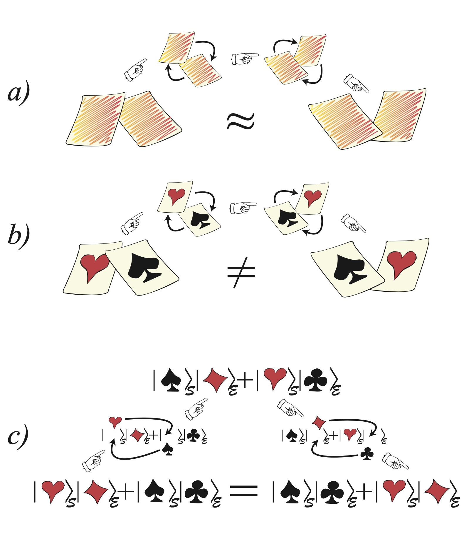
Consider again the maximally entangled state:

$$ \frac{1}{\sqrt{2}} (\mid \uparrow \uparrow \rangle + \mid \downarrow \downarrow \rangle) $$

If we act on the left with the $X$ operator, which swaps $\uparrow$ and $\downarrow$, we end up with:

$$X_{L}\frac{1}{\sqrt{2}} (\mid \uparrow \uparrow \rangle + \mid \downarrow \downarrow \rangle) \rightarrow \frac{1}{\sqrt{2}} (\mid \downarrow \uparrow \rangle + \mid \uparrow \downarrow \rangle) $$

The global state is transformed by this local action. But the original state can be restored by a "counterswap" on the right:

$$ X_{R} \frac{1}{\sqrt{2}} (\mid \downarrow \uparrow \rangle + \mid \uparrow \downarrow \rangle) \rightarrow \frac{1}{\sqrt{2}} (\mid \uparrow \uparrow \rangle + \mid \downarrow \downarrow \rangle) $$

So the global state is restored by an action another system. So we could say, if the global state is envariant under some unitary, then the individual subsystems must be invariant under that unitary. If a counterswap over there can undo a swap here, then what's being swapped or counterswapped can't be localized either here or there. Thus, insofar as the individual systems are invariant under local swaps, Laplace's principle of indifference applies, and we can say (objectively speaking) that $\uparrow$ and $\downarrow$ have equal likelihood.

The situation changes precisely because of entanglement. Classically, a perfect knowledge of the state of the whole implies perfect knowledge of the parts of that whole. But quantum mechanically, this is not generally the case! We can know precisely the state of the whole: i.e., that the two qubits are in the $\cup$ state, that they will be correlated in a particular way, while still being necessarily ignorant of the states of the individual qubits--not subjectively, but objectively. Indeed, knowing the global state is equivalent to knowing the correlations that will obtain between the two systems, but the envariance of the state, the fact that local swaps can be undone by swaps over there, implies that the local states themselves are invariant under swapping, and this objective indifference is the foundation for the probabilistic nature of quantum mechanics.

The same argument applies for $Y$ and $Z$ swaps.

Let's rewrite $ \frac{1}{\sqrt{2}} (\mid \uparrow \uparrow \rangle + \mid \downarrow \downarrow \rangle) $ in terms of $X$ eigenstates:

Recalling that $\mid \uparrow \rangle = \frac{1}{\sqrt{2}}(\mid \rightarrow \rangle + \mid \leftarrow \rangle)$ and $\mid \mid \downarrow \rangle = \frac{1}{\sqrt{2}}(\mid \rightarrow \rangle - \mid \leftarrow \rangle)$:

$$ \frac{1}{\sqrt{2}} (\mid \uparrow \uparrow \rangle + \mid \downarrow \downarrow \rangle) = \frac{1}{\sqrt{2}} \Bigg{(} \frac{1}{\sqrt{2}} \Big{\lbrack} \mid \rightarrow \rangle + \mid \leftarrow \rangle \Big{\rbrack} \frac{1}{\sqrt{2}} \Big{\lbrack} \mid \rightarrow \rangle + \mid \leftarrow \rangle \Big{\rbrack} + \frac{1}{\sqrt{2}} \Big{\lbrack} \mid \rightarrow \rangle - \mid \leftarrow \rangle \Big{\rbrack} \frac{1}{\sqrt{2}} \Big{\lbrack} \mid \rightarrow \rangle - \mid \leftarrow \rangle \Big{\rbrack} \Bigg{)}$$$$ = \frac{1}{\sqrt{2}} \Bigg{(} \frac{1}{2}\Big{\lbrack}\mid \rightarrow \rangle\mid \rightarrow \rangle + \mid \rightarrow \rangle\mid \leftarrow \rangle + \mid \leftarrow \rangle\mid \rightarrow \rangle + \mid \leftarrow \rangle\mid \leftarrow \rangle\Big{\rbrack} + \frac{1}{2}\Big{\lbrack} \mid \rightarrow \rangle\mid \rightarrow \rangle - \mid \rightarrow \rangle\mid \leftarrow \rangle - \mid \leftarrow \rangle\mid \rightarrow \rangle + \mid \leftarrow \rangle\mid \leftarrow \rangle\Big{\rbrack} \Bigg{)} $$$$= \frac{1}{\sqrt{2}}(\mid \rightarrow \rightarrow\rangle + \mid \leftarrow \leftarrow \rangle)$$

We can then consider the swap operator $\mid \rightarrow \rangle \langle \leftarrow \mid + \mid \leftarrow \rangle \langle \rightarrow \mid$, which is just Pauli $Z$ in disguise, and then the argument proceeds precisely as before, and we can derive the necessity of the 50/50 probabilities the $X$ direction as well. (And we could consider $Y$ swaps too.)

Notice also that these arguments don't work in the case of a single, isolated qubit. The most analogous case to Laplace's original example would be the case of two separable qubits: we're told one qubit is $\uparrow$ and one is $\downarrow$, we don't know which, but since swapping $\uparrow$ for $\downarrow$ doesn't make a difference, we should assign equal probabilities: but again, these are subjective probabilities. Entanglement is what makes all the difference.

But there's a catch, and it's that the argument from envariance under swaps only works to establish quantum probabilites on the basis of Laplace's principle of indifference when the coefficients are the same.

$$X_{L}(\alpha \mid \uparrow \uparrow \rangle + \beta \downarrow \downarrow \rangle) \rightarrow \alpha \mid \downarrow \uparrow \rangle + \beta \uparrow \downarrow \rangle$$

But:

$$X_{R}(\alpha \mid \downarrow \uparrow \rangle + \beta \mid \uparrow \downarrow \rangle) \rightarrow \alpha \mid \downarrow \downarrow \rangle + \beta \uparrow \uparrow \rangle$$

In other words, under a swap on the left and a swap on the right, a state with unequal coefficients doesn't return to itself: the coefficients switch places!

So the natural quesiton is whether we can generalize the above argument to the case of unequal coefficients.

In classical probability, there is the notion of "fine graining." Suppose I have two pebbles, one red and one blue, and I show you the red one $\frac{1}{3}$ of the time, and the blue one $\frac{2}{3}$ of the time. We could even things out, however, by imagining that we have three pebbles, one red and two blue, and I show them to you each $\frac{1}{3}$ of the time. The probabilities for "red" and "blue" in both cases are the same: $\frac{1}{3}$ and $\frac{2}{3}$. This is what is meant by finegraining. We take a situation where outcomes have uneven probabilities and reduce them to the case where there are more outcomes, which all have equal probability, and which are equivalent in the relevant sense to the original outcomes.

So that's what we're going to do in the quantum case.

Let's consider that we have a qubit, and we'll write its state like:

$$e^{i\phi_{a}}\sqrt{\frac{a}{n}}\mid \uparrow \rangle + e^{i\phi_{b}}\sqrt{\frac{b}{n}}\mid \downarrow \rangle $$

Where naturally $b = n-a$. We'll drop the phases, since they won't affect the general argument.

n = 3
a = np.random.randint(1,n)
b = n-a

print("n: %d, a: %s, b: %s" % (n, a, b))

alpha = np.exp(1j*0)*np.sqrt(a/n) 
beta = np.exp(1j*0)*np.sqrt(b/n)
qubit = alpha*qt.basis(2,0) + beta*qt.basis(2,1)

print("\nqubit:")
dirac(qubit)

n: 3, a: 1, b: 2

qubit:
0.577 |0> Pr: 0.333
0.816 |1> Pr: 0.667

Then let's entangle the qubit with a "measuring apparatus": in this case, just another qubit. The apparatus starts off in a known state: $\mid \uparrow \rangle$--and applying a a unitary CNOT leads to:

$$ \sqrt{\frac{a}{n}}\mid \uparrow \rangle_{S} \mid \uparrow \rangle_{A} + \sqrt{\frac{b}{n}}\mid \downarrow \rangle_{S} \mid \downarrow \rangle_{A}$$

from qutip.qip.operations import cnot

state = cnot()*qt.tensor(qubit, qt.basis(2,0))
dirac(state)

0.577 |00> Pr: 0.333
0.816 |11> Pr: 0.667

Now we consider that actually, our measuring apparatus is not in fact a qubit, but has tons of states: it's a complicated device. This is, of course, an eminently reasonable assumption. In fact, we'll assume it has at least $n$ possible states.

We'll then define a finegraining map for our apparatus:

$$ \mid \uparrow \rangle_{A} \rightarrow \frac{1}{\sqrt{a}}\sum_{i=0}^{a}\mid i \rangle_{A} $$$$ \mid \downarrow \rangle_{A} \rightarrow \frac{1}{\sqrt{b}}\sum_{i=a}^{b}\mid i \rangle_{A} $$

In other words, we imagine that what we were regarding as $\mid \uparrow \rangle_{A}$ is actually an even superposition of $a$ basis states of the apparatus, and what we were regarding as $\mid \downarrow \rangle_{A}$ is an even superposition of $b$ different basis states of the apparatus. These will still be orthogonal states.

fine_up = sum([qt.basis(n, i) for i in range(0, a)])/np.sqrt(a)
fine_down = sum([qt.basis(n, i) for i in range(a, n)])/np.sqrt(b)

fine_up, fine_down

(Quantum object: dims = [[3], [1]], shape = (3, 1), type = ket
 Qobj data =
 [[1.]
  [0.]
  [0.]],
 Quantum object: dims = [[3], [1]], shape = (3, 1), type = ket
 Qobj data =
 [[0.        ]
  [0.70710678]
  [0.70710678]])

In fact, this will be a unitary transformation.

First, we have it that $\mid \uparrow \rangle_{A}$ was secretly $\mid 0 \rangle_{A}$ and $\mid \downarrow \rangle_{A}$ was secretly $\mid 1 \rangle_{A}$, where $\mid 0 \rangle_{A}$ and $\mid 1 \rangle_{A}$ are just the first two of many basis states of the apparatus.

fine_grain = qt.basis(n,0)*qt.basis(2,0).dag() + qt.basis(n,1)*qt.basis(2,1).dag()
expanded = qt.tensor(qt.identity(2), fine_grain)*state

dirac(expanded)

0.577 |00> Pr: 0.333
0.816 |11> Pr: 0.667

We can then construct a unitary transformation that takes these two basis states to the even superpositions above.

m = np.zeros((n, n), dtype=complex)
m[:,0] = components(fine_up)
m[:,1] = components(fine_down)
R = -qt.Qobj(np.linalg.qr(m)[0])

print("R is unitary? %s" % np.allclose(R*R.dag(), qt.identity(n)))

R is unitary? True

fine_up, R*qt.basis(n,0)

(Quantum object: dims = [[3], [1]], shape = (3, 1), type = ket
 Qobj data =
 [[1.]
  [0.]
  [0.]],
 Quantum object: dims = [[3], [1]], shape = (3, 1), type = ket
 Qobj data =
 [[-1.]
  [ 0.]
  [ 0.]])

fine_down, R*qt.basis(n,1)

(Quantum object: dims = [[3], [1]], shape = (3, 1), type = ket
 Qobj data =
 [[0.        ]
  [0.70710678]
  [0.70710678]],
 Quantum object: dims = [[3], [1]], shape = (3, 1), type = ket
 Qobj data =
 [[0.        ]
  [0.70710678]
  [0.70710678]])

fine_grained = qt.tensor(qt.identity(2), R)*expanded
dirac(fine_grained)

-0.577 |00> Pr: 0.333
0.577 |11> Pr: 0.333
0.577 |12> Pr: 0.333

In other words, our state is now:

$$ \sqrt{\frac{a}{n}}\mid \uparrow \rangle_{S} \frac{1}{\sqrt{a}}\sum_{i=0}^{a}\mid i \rangle_{A} + \sqrt{\frac{b}{n}}\mid \downarrow \rangle_{S} \frac{1}{\sqrt{b}}\sum_{i=a}^{b}\mid i \rangle_{A}$$

Or:

$$ \frac{1}{\sqrt{n}}\Bigg{(}\sum_{i=0}^{a}\mid \uparrow \rangle_{S} \mid i \rangle_{A} + \sum_{i=a}^{b}\mid \downarrow \rangle_{S}\mid i \rangle_{A} \Bigg{)} $$

And so we've converted unequal coefficients into equal coefficients.

But we're not done yet. To make our envariance argument, we need to be able to do unitary swaps and counterswaps. But you'll find if you try to construct such a swap on the apparatus, it won't be unitary--and if you try to force it to be (via a QR decomposition), then it won't give you the right transformation.

bad_swap = fine_up*fine_down.dag() + fine_down*fine_up.dag()
bad_swap_unitary = -qt.Qobj(np.linalg.qr(bad_swap.full())[0])

fine_up, bad_swap_unitary*fine_down

(Quantum object: dims = [[3], [1]], shape = (3, 1), type = ket
 Qobj data =
 [[1.]
  [0.]
  [0.]],
 Quantum object: dims = [[3], [1]], shape = (3, 1), type = ket
 Qobj data =
 [[-0.70710678]
  [ 0.5       ]
  [-0.5       ]])

fine_down, bad_swap_unitary*fine_down

(Quantum object: dims = [[3], [1]], shape = (3, 1), type = ket
 Qobj data =
 [[0.        ]
  [0.70710678]
  [0.70710678]],
 Quantum object: dims = [[3], [1]], shape = (3, 1), type = ket
 Qobj data =
 [[-0.70710678]
  [ 0.5       ]
  [-0.5       ]])

Clearly, it doesn't work. So actually, we're going to introduce a third system: the "environment" in which the apparatus and system are immersed, and which gets entangled with them. Just think of it like yet another link in the chain of entanglement.

$$ \frac{1}{\sqrt{n}}\Bigg{(}\sum_{i=0}^{a}\mid \uparrow \rangle_{S} \mid i \rangle_{A} \mid i \rangle_{E} + \sum_{i=a}^{b}\mid \downarrow \rangle_{S}\mid i \rangle_{A} \mid i \rangle_{E} \Bigg{)} $$

Then we can do unitary swaps on the qubit + apparatus, which can be unswapped on the environment alone.

qubit_app_env = (sum([qt.tensor(qt.basis(2,0), qt.basis(n, i), qt.basis(n, i)) for i in range(a)]) +\
                 sum([qt.tensor(qt.basis(2,1), qt.basis(n, i), qt.basis(n, i)) for i in range(a, n)])).unit()

dirac(qubit_app_env)

0.577 |000> Pr: 0.333
0.577 |111> Pr: 0.333
0.577 |122> Pr: 0.333

So let's choose a random basis state between $0$ and $a$ on the qubit + environment to swap with a random basis state between $a$ and $n$.

k, l = np.random.randint(0, a), np.random.randint(a, n)
print("swapping: %d, %d" % (k, l))

swapping: 0, 2

And then construct a unitary swap operator:

sys_app_swap = qt.tensor(qt.basis(2,1), qt.basis(n, l))*qt.tensor(qt.basis(2,0), qt.basis(n, k)).dag() +\
               qt.tensor(qt.basis(2,0), qt.basis(n, k))*qt.tensor(qt.basis(2,1), qt.basis(n, l)).dag()
sys_app_swap = -qt.Qobj(np.linalg.qr(sys_app_swap.full())[0])

print("sys_app_swap unitary? %s" % np.allclose(sys_app_swap*sys_app_swap.dag(), qt.identity(2*n)) )
sys_app_swap.dims = [[2, n], [2, n]]

sys_app_swap unitary? True

Let's check that it acts correctly:

qt.tensor(qt.basis(2,1), qt.basis(n, l)), sys_app_swap*qt.tensor(qt.basis(2,0), qt.basis(n, k))

(Quantum object: dims = [[2, 3], [1, 1]], shape = (6, 1), type = ket
 Qobj data =
 [[0.]
  [0.]
  [0.]
  [0.]
  [0.]
  [1.]],
 Quantum object: dims = [[2, 3], [1, 1]], shape = (6, 1), type = ket
 Qobj data =
 [[0.]
  [0.]
  [0.]
  [0.]
  [0.]
  [1.]])

qt.tensor(qt.basis(2,0), qt.basis(n, k)), sys_app_swap*qt.tensor(qt.basis(2,1), qt.basis(n, l))

(Quantum object: dims = [[2, 3], [1, 1]], shape = (6, 1), type = ket
 Qobj data =
 [[1.]
  [0.]
  [0.]
  [0.]
  [0.]
  [0.]],
 Quantum object: dims = [[2, 3], [1, 1]], shape = (6, 1), type = ket
 Qobj data =
 [[1.]
  [0.]
  [0.]
  [0.]
  [0.]
  [0.]])

And then let's construct the environment swap operator:

env_swap = qt.basis(n, l)*qt.basis(n, k).dag() + qt.basis(n, k)*qt.basis(n, l).dag()
env_swap = -qt.Qobj(np.linalg.qr(env_swap.full())[0])

print("env_swap unitary? %s" % np.allclose(env_swap*env_swap.dag(), qt.identity(n)))

env_swap unitary? True

And check that it acts correctly:

qt.basis(n, l), env_swap*qt.basis(n, k)

(Quantum object: dims = [[3], [1]], shape = (3, 1), type = ket
 Qobj data =
 [[0.]
  [0.]
  [1.]],
 Quantum object: dims = [[3], [1]], shape = (3, 1), type = ket
 Qobj data =
 [[0.]
  [0.]
  [1.]])

qt.basis(n, k), env_swap*qt.basis(n, l)

(Quantum object: dims = [[3], [1]], shape = (3, 1), type = ket
 Qobj data =
 [[1.]
  [0.]
  [0.]],
 Quantum object: dims = [[3], [1]], shape = (3, 1), type = ket
 Qobj data =
 [[1.]
  [0.]
  [0.]])

And finally, putting it together:

swap = qt.tensor(sys_app_swap, qt.identity(n))
counter_swap = qt.tensor(qt.identity(2), qt.identity(n), env_swap)

print("starting off...")
dirac(qubit_app_env)
print()
print("swapping on qubit/apparatus...")
dirac(swap*qubit_app_env)
print()
print("counterswapping on environment...")
dirac(counter_swap*qubit_app_env)
print()
print("swap and counterswap:")
dirac(swap*counter_swap*qubit_app_env)

starting off...
0.577 |000> Pr: 0.333
0.577 |111> Pr: 0.333
0.577 |122> Pr: 0.333

swapping on qubit/apparatus...
0.577 |002> Pr: 0.333
-0.577 |111> Pr: 0.333
0.577 |120> Pr: 0.333

counterswapping on environment...
0.577 |002> Pr: 0.333
-0.577 |111> Pr: 0.333
0.577 |120> Pr: 0.333

swap and counterswap:
0.577 |000> Pr: 0.333
0.577 |111> Pr: 0.333
0.577 |122> Pr: 0.333

So swaps between states on the system/apparatus can be undone by swaps on the environment, and thus by the invariance argument, we have to regard each outcome as being equiprobable. And because of our fine graining, this amounts to qubit outcomes with the desired unequal probabilities.

So let's discuss the plausibility of this argument, which may at first seem somewhat contrived.

On the one hand, it's quite natural to regard the measuring apparatus to have many states, and it's also quite natural to include the environment with many states as well into the picture, and to suppose that there will be a chain of maximal entanglement. What does seem strange is the part where we choose a special unitary transformation that seems to depend on the specific amplitudes of the state! It all worked because our amplitudes were $\sqrt{\frac{a}{n}}$ and $\sqrt{\frac{b}{n}}$, and we transformed to a basis where the qubit was entangled with an even superposition of $a$ basis states and an even superposition of $b$ basis states. Are we supposed to imagine that this transformation is really taking place; and what's more, is somehow sensitive to the amplitudes of the qubit themselves?

One could say, and Zurek does say, that the important thing is that such a transformation is possible: it's a unitary transformation, and so we're perfectly within our rights to redescribe the state, and so characterize the entanglement in those terms. In other words, the state is such that, if we do describe it in this basis, then Born's rule for probabilities comes out naturally by envariance. This is an objective property of the state even if such a transformation isn't applied in the step-by-step way I laid out above. After all, we aren't using any old unitary on the system as a whole, which would trivially allow us to prove anything--we're just doing a basis shift on the apparatus (and environment)--which crucially, doesn't affect the entanglement at all.

On the other hand, it's not impossible that such conditions do actually obtain in any realistic measurement set-up, and that these are precisely the conditions we're satisfying when we do successfully measure a quantum system, even if we didn't know that's what we were doing! This is an interesting question to settle experimentally.

It also connects up with Zurek's other work on einselection and decoherence, which provides an analysis of how certain basis states (pointer states) come to be preferred by the continuous monitoring of a system by the environment. A pointer basis corresponds to an operator which commutes with the interaction Hamiltonian, and so that over time, due to decoherence, the density matrix of the system becomes diagonal in precisely that basis. It's also worth considering his other work on "Quantum Darwinism," which is an analysis of how interactions with the environment lead to a kind of natural selection, whereby "classical" information about systems is able to reproduce itself in that environment, from which the original state can be reconstructed, giving the appearance of classical objectivity--after all, all our measurements are indirect reconstructions of this type.

What if the apparatus doesn't have $n$ basis states? What happens then? Well, maybe those are the apparatuses we characterize as defective! After all, what we're really talking about is trying to characterize the amplitudes up to a certain accuracy. The same kind of argument can apply to the objection that sometimes irrational numbers may appear as amplitudes.

Finally, in what sense does this resolve the "collapse" issue? I think this can go in several different directions. On the one hand, one could use the envariance argument to support a Many-Worlds type picture, insofar as the envariance + finegraining argument obviates the usual objection that "if all possibilities really occur" then what role do the probabilities even serve? Here the probabilities are grounded operationally in the objective indifference under swaps and counterswaps, and because of the fine graining, it's perfectly fine to "count the number of branches," and reason that there are more worlds/versions of you that encounter this outcome or that. In a sense, the probabilities could be seen as referring to "which branch you'll find yourself in."

On the other hand, I think the same arguments can also support a relational interpretation of quantum mechanics (and actually, in the end, I think these two interpretations are probably complementary to each other, the former emphasizing the global picture, and the the latter emphasizing the local). A maximally entangled state fully characterizes the correlations between two systems, leaving their individual states (in the case of spin, their orientations) undetermined. Another way of thinking about this is that the two systems have a perfectly definite orientation relative to each other, but no definite orientation to you. Thus when you force one of the systems to have a definite orientation relative to you by measurement, the result is random: but the two pictures of the world are made consistent by the entanglement, so that after your measurement, the qubits still agree. Now you and the spins have a definite relation to each other, but from another point of view, not part of this relation, you're all entangled and indeterminant. But one should be careful here in using phrases like "from another perspective" or "from a 1st person vs a 3rd person perspective." By perspective we can mean many things, of which I'd like to distinguish three: a) our inner life, b) what we actually see with our eyes, c) the physical state of the world relative to us. Famously, special relativity predicts length contraction of objects in the direction of their motion, which of course, depends on the relative motion between you and the object. Ironically, this effect is actually invisible to the eye because if you follow the trajectories of light rays from the object, optical effects perfectly cancel out the relativistic effect. But by other evidence, from particle interactions, and so forth, it can be shown that length contraction really does effect the physics of things "from your perspective." In other words, we all have a "perspective" on the physical world, which is different from our perspective in the subjective sense (or the optical sense). In other words, there is both a subjective and an objective kind of perspective, and it's in this latter sense that one can say, from a 1st person perspective, a definite outcome occurs with a certain probability, while from a 3rd person perspective, unitary evolution continues apace. The cleverness of the envariance argument is to derive the 1st person probability from the 3rd person entanglement.