On the impossibility of "stealth communication"
Suppose we have a spin-$\frac{1}{2}$ state pointed in the $X+$ direction, and we've quantized along the $Z$ axis.
We can represent this state as a ket: e.g., $\mid \phi \rangle = \frac{1}{\sqrt{2}} (\mid \uparrow \rangle + \mid \downarrow \rangle)$, and expand it out as a two dimensional complex vector: $\begin{pmatrix} \frac{1}{\sqrt{2}} \\ \frac{1}{\sqrt{2}} \end{pmatrix}$.
We could also represent the state as a density matrix, given by an outer product:
$\mid \phi \rangle \langle \phi \mid = \begin{pmatrix} \frac{1}{2} & \frac{1}{2} \\ \frac{1}{2} & \frac{1}{2} \end{pmatrix}$.
One thing that's nice about a density matrix is that the probabilities for the results of a $Z$ measurement are just given by the diagonal elements. If we send this state through a Stern-Gerlach oriented along the $Z$ axis, it'll give $\mid \uparrow \rangle$ half the time, and $\mid \downarrow \rangle$ half the time.
Nevertheless, this density matrix still represents a pure state. Mathematically, this means that the matrix, in fact, is a rank-1 matrix, which means that it can be written as a simple outer product, as we've done. This particular pure state is a superposition of $\mid \uparrow \rangle$ and $\mid \downarrow \rangle$, so that if we measure along the $Z$ direction, there is intrinsic quantum uncertainty about which answer we will obtain. On the other hand, if we measure along the $X$ direction, we'll get $\mid \uparrow \rangle$ 100% of the time.
Suppose, however, we didn't know exactly which state we were working with, not because of quantum uncertainty, but because of just normal, classical, epistemic ignorance. For example, perhaps we had reason to believe that the state in question was equally likely to be $\mid \phi \rangle = \frac{1}{\sqrt{2}} (\mid \uparrow \rangle + \mid \downarrow \rangle)$ or $\mid \psi \rangle = \frac{1}{\sqrt{2}} (\mid \uparrow \rangle - \mid \downarrow \rangle)$, but we simply didn't know which one.
We can represent this situation as a proper mixed state, a sum of pure state density matrices weighted by probabilities.
Since $\mid \phi \rangle \langle \phi \mid = \begin{pmatrix} \frac{1}{2} & \frac{1}{2} \\ \frac{1}{2} & \frac{1}{2} \end{pmatrix}$ and $\mid \psi \rangle \langle \psi \mid = \begin{pmatrix} \frac{1}{2} & -\frac{1}{2} \\ -\frac{1}{2} & \frac{1}{2} \end{pmatrix}$, we'd obtain:
$ \frac{1}{2} \mid \phi \rangle \langle \phi \mid + \frac{1}{2} \mid \psi \rangle \langle \psi \mid = \frac{1}{2} \begin{pmatrix} \frac{1}{2} & \frac{1}{2} \\ \frac{1}{2} & \frac{1}{2} \end{pmatrix} + \frac{1}{2} \begin{pmatrix} \frac{1}{2} & -\frac{1}{2} \\ -\frac{1}{2} & \frac{1}{2} \end{pmatrix} = \begin{pmatrix} \frac{1}{2} & 0 \\ 0 & \frac{1}{2} \end{pmatrix}$.
This density matrix is a mixed state, in fact, a maximally mixed state. Mathematically, it is a rank-2 matrix: it can't be written as an outer product, but only as a weighted sum of outer products.
In other words, we don't know whether we're dealing with a $\mid \rightarrow \rangle$ state or a $\mid \leftarrow \rangle$ state; but what we can say is that if we send whatever it is through a Stern-Gerlach oriented in the $Z$ direction, we'll get $\mid \uparrow \rangle$ or $\mid \downarrow \rangle$ with equal probability. And in this case, we get the same if instead we measure the $X$ direction (or the $Y$ direction, for that matter).
Although a mixed state must be written as a sum of outer products, it can be written as a sum of outer products in many different ways. For example, if we had $\frac{1}{2} \mid \uparrow \rangle \langle \uparrow \mid + \frac{1}{2}\mid \downarrow \rangle \langle \downarrow \mid$, we'd obtain the same density matrix: $\begin{pmatrix} \frac{1}{2} & 0 \\ 0 & \frac{1}{2} \end{pmatrix}$.
In other words, using a Stern-Gerlach, we can't distinguish between the case where we had $\mid \leftarrow \rangle$ or $\mid \rightarrow \rangle$ from the case where we had $\mid \uparrow \rangle$ or $\mid \downarrow \rangle$. Mathematically, this is encoded in the fact that the same mixed state describes both cases.
In other words, if we run many identically prepared such mixtures through Stern-Gerlachs, we'll be able to deduce that the probabilites are $\frac{1}{2}$ and $\frac{1}{2}$ for $\mid \uparrow \rangle$ and $\mid \downarrow \rangle$ (or $\mid \leftarrow \rangle$ or $\mid \rightarrow \rangle$), but in this case, we'll remain maximally ignorant about which direction the spin was originally pointed in. This situation of maximal ignorance is mathematically represented in the fact that the off-diagonal terms of the density matrix are all 0.
This, however, is not the only way that mixed states can arise.
Suppose we have two spin-$\frac{1}{2}$ particles $A$ and $B$ in the antisymmetric state: $\frac{1}{\sqrt{2}} (\mid \uparrow \downarrow \rangle - \mid \downarrow \uparrow \rangle)$, also known as the singlet state.
This is a state in the tensor product $H_{A} \otimes H_{B}$, where $H_{A}$ and $H_{B}$ are the Hilbert spaces for the individual spin-$\frac{1}{2}$'s. The standard basis set for the tensor product is given by: $\mid \uparrow \uparrow \rangle, \mid \uparrow \downarrow \rangle, \mid \downarrow \uparrow \rangle, \mid \downarrow \downarrow \rangle$.
Expanding in this basis, we can represent the state as a 4 dimensional complex vector: $\begin{pmatrix} 0 \\ \frac{1}{\sqrt{2}} \\ -\frac{1}{\sqrt{2}} \\ 0 \end{pmatrix}$.
This is, in fact, an entangled state. In other words, it can't be written as a single tensor product of an $A$ state and a $B$ state, but only as a sum of such states. Because of this, we can't associate pure states to $A$ and $B$ individually, but only a pure state to them together (even if they happen to be spatially separate).
For this particular state, $A$ and $B$ each have a 50% chance of being $\uparrow$ or $\downarrow$ in whatever direction we choose to measure in, but also: if they are measured in the same directions, they will always be found to be pointing opposite to each other.
Just as before, we can associate a pure density matrix to this state: $\begin{pmatrix} 0 & 0 & 0 & 0 \\ 0 & \frac{1}{2} & -\frac{1}{2} & 0 \\ 0 & -\frac{1}{2} & \frac{1}{2} & 0 \\ 0 & 0 & 0 & 0 \end{pmatrix}$.
Now here's the thing: even though we can't assign pure states to $A$ and $B$ individually, we can nevertheless encode the information available locally at $A$ and the information available locally at $B$ in the form of two improper mixed states. These states are obtained by taking a "partial trace" of the pure state density matrix of the two together.
If we have a pure state density matrix $\rho_{AB} = \sum_{ijkl} c_{ijkl} \mid a_{i} \rangle \langle a_{j} \mid \otimes \mid b_{k} \rangle \langle b_{l} \mid$, then the partial trace over $B$, which gives $\rho_{A}$ is:
$\rho_{A} = \sum_{ijkl} c_{ijkl}\mid a_{i} \rangle \langle a_{j} \mid \langle b_{l}\mid b_{k} \rangle$
Similarly:
$\rho_{B} = \sum_{ijkl} c_{ijkl} \langle a_{i} \mid a_{j} \rangle \mid b_{l}\rangle \langle b_{k} \mid$
In the case of two spin-$\frac{1}{2}$ states, taking the partial trace is quite easy.
$\rho_{A} = tr_{B}(\rho_{AB}) = tr_{B} \begin{pmatrix} a & b & c & d \\ e & f & g & h \\ i & j & k & l \\ m & n & o & p \end{pmatrix} = \begin{pmatrix} tr \begin{pmatrix} a & b \\ e & f \end{pmatrix} & tr \begin{pmatrix} c & d \\ g & h \end{pmatrix} \\ tr \begin{pmatrix} i & j \\ m & n \end{pmatrix} & tr \begin{pmatrix} k & l \\ o & p \end{pmatrix} \end{pmatrix} = \begin{pmatrix} a + f & c + h \\ i + n & k + p \end{pmatrix}$
$\rho_{B} = tr_{A}(\rho_{AB}) = tr_{A} \begin{pmatrix} a & b & c & d \\ e & f & g & h \\ i & j & k & l \\ m & n & o & p \end{pmatrix} = \begin{pmatrix} tr \begin{pmatrix} a & c \\ i & k \end{pmatrix} & tr \begin{pmatrix} b & d \\ j & l \end{pmatrix} \\ tr \begin{pmatrix} e & g \\ m & o \end{pmatrix} & tr \begin{pmatrix} f & h \\ n & p \end{pmatrix} \end{pmatrix} = \begin{pmatrix} a + k & b + l \\ e + o & f + p \end{pmatrix}$
Another nice way of thinking about the partial trace is in terms of string diagrams (nothing to do with string theory!). If we define $\mid \cup \rangle = \mid \uparrow \uparrow \rangle + \mid \downarrow \downarrow \rangle$, and $\langle \cap \mid = \langle \uparrow \uparrow \mid + \langle \downarrow \downarrow \mid$, we can represent the partial state of $A$ as:
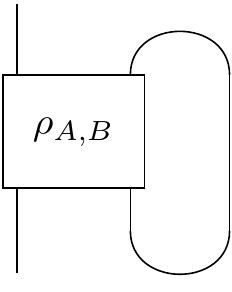
In other words, $ \rho_{A} = \big( I \otimes \cap \big) \big(\rho_{AB} \otimes I \big) \big( I \otimes \cup \big) $.
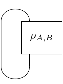
Aka: $ \rho_{B} = \big( \cap \otimes I \big) \big( I \otimes \rho_{AB} \big) \big( \cup \otimes I \big) $.
In our case, $\rho_{AB} = \begin{pmatrix} 0 & 0 & 0 & 0 \\ 0 & \frac{1}{2} & -\frac{1}{2} & 0 \\ 0 & -\frac{1}{2} & \frac{1}{2} & 0 \\ 0 & 0 & 0 & 0 \end{pmatrix}$.
And so, we find that the partial state of $A$ is $\begin{pmatrix} \frac{1}{2} & 0 \\ 0 & \frac{1}{2} \end{pmatrix}$, and the partial state of $B$ is $\begin{pmatrix} \frac{1}{2} & 0 \\ 0 & \frac{1}{2} \end{pmatrix}$.
In other words, the partial states of $A$ and $B$ are both maximally mixed states. These mixed states are both "improper mixtures" in that they are reduced states of an overall entangled pure state of the two spins.
Interestingly, whereas there are non-zero off-diagonal terms in the pure state density matrix of $A$ and $B$ together, representing the fact that the joint state is a superposition, the off-diagonal terms of the partial states are all 0. In other words, these partial states cannot be described as quantum superpositions individually, but instead must be described as mixtures, lacking any "quantum coherence."
For simplicity, let's assume that Alice (who has $A$) and Bob (who has $B$) both agree to measure their particle in the $Z$ direction.
Suppose Bob goes first and measures his spin. Half the time Bob will get $\mid \uparrow \rangle$ and half the time Bob will get $\mid \downarrow \rangle$.
Mathematically, we can represent this as a projection: we act with either $I \otimes \mid \uparrow \rangle \langle \uparrow \mid$ or $I \otimes \mid \downarrow \rangle \langle \downarrow \mid$ on the singlet (and then normalize).
In the first case, the joint state will end up as: $\mid \downarrow \rangle \mid \uparrow \rangle$ or $\begin{pmatrix} 0 \\ 0 \\ 1 \\ 0 \end{pmatrix}$.
In the second case, the joint state will end up as $\mid \uparrow \rangle \mid \downarrow \rangle$ or $\begin{pmatrix} 0 \\ 1 \\ 0 \\ 0 \end{pmatrix}$.
In both cases, we end up with $A$ and $B$ in separable states.
If we consider the state of $A$ after Bob's measurement of $B$, we have a situation of classical, epistemic uncertainty with regard to whether $A$ is now $\mid \uparrow \rangle$ or $\mid \downarrow \rangle$. In other words, $A$'s state is a proper mixture: $\frac{1}{2}\mid \uparrow \rangle \langle \uparrow \mid + \frac{1}{2}\mid \downarrow \rangle \langle \downarrow \mid$, i.e.: $\begin{pmatrix} \frac{1}{2} & 0 \\ 0 & \frac{1}{2} \end{pmatrix}$.
But notice, that's just the same density matrix for $A$ as before Bob's measurement of $B$!
Indeed, we can see that whether or not Bob makes a measurement of $B$, the density matrix for $A$ is precisely the same: the maximally mixed state. In the first case, the maximally mixed state is an "improper mixture," being the reduced state of one half of a pure entangled state. In the second case, the maximally mixed state is a "proper mixture," representing the classical uncertainty with regard to whether $A$ has ended up $\mid \uparrow \rangle$ or $\mid \downarrow \rangle$. But either way, it's the same density matrix.
The consequence is that there is absolutely no effect local to $A$ that can reveal whether or not Bob has made a measurement on $B$.
Indeed, consider the following. If Bob does make a measurement, then Alice ends up with a proper mixed state. As we've said, this state doesn't so much represent the "actual" state of the particle as Alice's ignorance about whether her spin has collapsed to $\mid \uparrow \rangle$ or $\mid \downarrow \rangle$ due to Bob's measurement. The point is that even if the spin has collapsed to being the one or the other, there is no way for Alice to know what it has collapsed to unless she herself does a measurement (or Bob phones her up and tells her). For example, you might say: well, if the spin has collapsed to $\mid \uparrow \rangle$ due to Bob's measurement, then if Alice measures along the $Z$ axis, it'll be $\mid \uparrow \rangle$ 100% of the time; but remember Alice has only one shot at measurement, and each time the experiment is repeated, she gets $\mid \uparrow \rangle$ or $\mid \downarrow \rangle$ at random just as Bob's result is random. If she doesn't know about Bob at all, maybe she thinks she has the unentangled state $\mid \uparrow \rangle + \mid \downarrow \rangle$. So she tries measuring along the $X$ axis instead: but again, it's 50/50: since that's what happens if you measure a $Z$ eigenstate along the $X$ axis. And then she tries the $Y$ axis, and it's 50/50, for the same reason. This is precisely what the maximally mixed state represents.
But here's the subtlety. Suppose Alice herself makes a measurement. It's possible that some relativistic observer will say she did her measurement before Bob, but another observer might say that Bob did his measurement before Alice. In other words, depending on one's time ordering of events, one would classify Alice's maximally mixed state as an improper mixture (if she measures first) or a proper mixture (if Bob measures first). But it doesn't matter because the density matrix is the same either way!
Indeed, it makes no difference whether Alice or Bob measures first; the relationship is completely symmetrical. Their answers ($\uparrow$ or $\downarrow$) are always random, and the answers always (dis)agree. The correlations can only be noticed by doing measurements on both particles, and bringing the results together and comparing them, and doing this many, many times. There is no way to tell which entangled state the particles are in by subjecting them individually to local measurements without later comparing the results, and there's no way to tell locally whether Bob (or Alice) has already measured his (or her) particle first. Given a singlet state, whether or not Bob/Alice has made a measurement, Alice/Bob's description of the particle before her/his own measurement is necessarily the same: the maximally mixed state.
Finally, a word on the relationship between "interference" and the tensor product.
In the classic double slit experiment, the wave function of a particle propagates towards two slits, goes through both, and interferes with itself: we end up in a state like $\mid upper \ path \rangle + \mid lower \ path \rangle$. Therefore, when we measure the particle's position against a screen, we get an interference pattern of bands of light and dark.
But suppose we put detectors by the two slits, and snoop on which path the particle "actually takes." The effect of this is that we instead end up in a state like: $\mid upper \ path \ detected \rangle \mid upper \ path \rangle + \mid lower \ path \ detected \rangle\mid lower \ path \rangle$.
This is a state in the tensor product of the detector and the particle's position.
By construction, the states $\mid upper \ path \ detected \rangle$ and $\mid lower \ path \ detected \rangle$ are orthogonal with each other: $\langle upper \ path \ detected \mid lower \ path \ detected \rangle = 0$. Therefore, the two tensor product states $\mid upper \ path \ detected \rangle \mid upper \ path \rangle$ and $\mid lower \ path \ detected \rangle \mid lower \ path \rangle$ are also orthogonal to each other, regardless of what $\mid upper \ path \rangle$ and $ \mid lower \ path \rangle$ happen to be. This is how the tensor product works. Therefore, when you add the two tensor products together, there will be no interference in position. The tensor product is "big enough" to keep the two position states separate from each other.
In "Many Worlds" terminology, the two position states are propagating in "different worlds," kept separate by the two states of the detector, one world associated with $ \mid upper \ path \ detected \rangle $ and another world associated with $\mid lower \ path \ detected \rangle $. The effect is that if you add detectors sensitive to which path the particle took, then the interference pattern dissapears.
The same applies to a particle with spin being sent through a Stern-Gerlach, say, oriented in the $Z$ direction. The apparatus functions by entangling the position and spin of the particle so that afterwards the state of the particle is something like: $\mid spin \uparrow \rangle \mid upper \ path \rangle + \mid spin \downarrow \rangle \mid lower \ path \rangle$. Just as in the former case, the two spin states $\mid \uparrow \rangle$ and $\mid \downarrow \rangle$ are at right angles, and so the two states in the superposition are also at right angles, and thus when they are added, there is no interference in position, if, for example, we put a double slit after a Stern-Gerlach. The spin of the particle, in other words, encodes "which way" information, and so there is no interference in the two "beams" that exit from a Stern-Gerlach. In other words, even if the original spin state is in a superposition, and so "comes out both ports of the Stern-Gerlach," these two beams won't interfere with each other in terms of their position.
On the other hand, suppose we send those two beams through another Stern-Gerlach, this time oriented in the $X$ direction. (Here, I follow nice paper.)
After the first Stern-Gerlach, we're in the state: $\mid \uparrow \rangle \mid upper \ path \rangle + \mid \downarrow \rangle \mid lower \ path \rangle$.
Let's rewrite this in terms of $X$ eigenstates:
$(\mid \rightarrow \rangle + \mid \leftarrow \rangle)\mid upper \ path \rangle + (\mid \rightarrow \rangle - \mid \leftarrow \rangle)\mid lower \ path \rangle$.
We can engage in a little algebra:
$\mid \rightarrow \rangle\mid upper \ path \rangle + \mid \leftarrow \rangle\mid upper \ path \rangle + \mid \rightarrow \rangle\mid lower \ path \rangle - \mid \leftarrow \rangle\mid lower \ path \rangle$
$ \mid \rightarrow \rangle(\mid upper \ path \rangle + \mid lower \ path \rangle) + \mid \leftarrow \rangle(\mid upper \ path \rangle - \mid lower \ path \rangle)$
We can see that the interference pattern can to some extent be recovered. In fact, if we do this experiment many times, against the back wall, we'll observe two offset interference patterns side by side, $\mid upper \ path \rangle + \mid lower \ path \rangle$, associated with $\mid \rightarrow \rangle$, and $\mid upper \ path \rangle - \mid lower \ path \rangle$, associated with $\mid \leftarrow \rangle$. The second Stern-Gerlach has effective "erased" the which-way information, and so restored the interference in position.
Another thing worth considering, which we've already somewhat implied, is the analogous situation for just the spin state. A spin in a superposition $\alpha \mid \uparrow \rangle + \beta \mid \downarrow \rangle$ is sent through a Stern-Gerlach, and ends up in the entangled state: $\alpha \mid \uparrow \rangle\mid upper \ path \rangle + \beta \mid \downarrow \rangle\mid lower \ path \rangle$. If we measure the position of the particle afterwards, we'll find that the position is always correlated to the spin, and so we might imagine that, in fact, only the $\uparrow$ part or the $\downarrow$ part actually made it through the apparatus, each with a certain probability, and ended up along the up or down paths. On the other hand, if instead of measuring the position, we allow the two beams to recombine, we can recover the original superposition of spin states $\alpha \mid \uparrow \rangle + \beta \mid \downarrow \rangle$, which we can confirm by sending it through another Stern-Gerlach (and doing this experiment many times). In this latter case, we'd thus have to regard the spin as exiting both ports of the apparatus. In this case, we're recovering the "coherence" or "interference" for the spin, not the position. And in the case of a spin, recovering the original "coherence" or "interference pattern" just means recovering the original direction that the spin was pointed in.
Finally, what happens if we use our "which path" eraser on one half of a singlet state?
In terms of the spins, we start with:
$\mid \uparrow \rangle_{A} \mid \downarrow \rangle_{B} - \mid \downarrow \rangle_{A} \mid \uparrow \rangle_{B}$
We then send $B$ through the first $Z$ Stern-Gerlach:
$\mid \uparrow \rangle_{A} \mid \downarrow \rangle_{B} \mid down \ path \rangle_{B} - \mid \downarrow \rangle_{A} \mid \uparrow \rangle_{B} \mid up \ path \rangle_{B}$
We then send $B$ through the $X$ Stern-Gerlach. Rewriting in terms of $X$ eigenstates:
$\mid \uparrow \rangle_{A} (\mid \leftarrow \rangle - \mid \rightarrow \rangle)_{B} \mid down \ path \rangle_{B} - \mid \downarrow \rangle_{A} (\mid \leftarrow \rangle + \mid \rightarrow \rangle)_{B} \mid up \ path \rangle_{B}$
Rearranging terms, we eventually obtain:
$ \mid \rightarrow \rangle_{B}\big{(}\mid down \ path \rangle_{B}\mid \uparrow \rangle_{A} - \mid up \ path \rangle_{B}\mid \downarrow \rangle_{A}\big{)} + \mid \leftarrow \rangle_{B}\big{(}\mid up \ path \rangle_{B}\mid \downarrow \rangle_{A} - \mid down \ path \rangle_{B}\mid \uparrow \rangle_{A}\big{)}$
We can therefore see that we won't obtain any interference pattern in $B$'s position, since $A$'s $\mid \uparrow \rangle$ and $\mid \downarrow \rangle$ states keep $B$'s up and down path states separate.
What if we measure $A$ to be $\uparrow$? Well, let's work it out just to be sure:
$ \mid \rightarrow \rangle_{B}\mid down \ path \rangle_{B}\mid \uparrow \rangle_{A} - \mid \leftarrow \rangle_{B} \mid down \ path \rangle_{B}\mid \uparrow \rangle_{A}$
$(\mid \rightarrow \rangle_{B} - \mid \leftarrow \rangle_{B} ) \mid down \ path \rangle_{B}\mid \uparrow \rangle_{A}$
$\mid \downarrow \rangle_{B} \mid down \ path \rangle_{B}\mid \uparrow \rangle_{A}$
Conversely, we'd get $\mid \uparrow \rangle_{B} \mid up \ path \rangle_{B}\mid \downarrow \rangle_{A}$ if $A$ had been measured to be $\downarrow$.
Either way: no interference. So we can't use the presence or absence of interference to determine whether $A$ has made a measurement or not.