More Fun with Coherent States
We've seen coherent states in the context of the quantum harmonic oscillator as well as for quantum spins. It's worth thinking about an even simpler example. I follow the excellent work of J. P. Gazeau in what follows.
We'll be taking as our Hilbert space the circle, in fact, ultimately, the circle with opposite points identified. In other words: the space of oriented lines in the plane. This is a two-dimensional real Hilbert space.
For example, we all know we can specify a point on a 2D plane in terms of $x$ and $y$ coordinates. Since we're restricting to the unit circle, we could also parameterize the point solely by its angle: $\theta$.
We could take as our basis vectors $\mid 0 \rangle = \begin{pmatrix} 1 \\ 0 \end{pmatrix}$ and $\mid \frac{\pi}{2} \rangle = \begin{pmatrix} 0 \\ 1 \end{pmatrix}$.
The notation $\mid \theta \rangle$ means a unit vector with angle $\theta$, between $0$ and $2\pi$. Our two basis states clearly resolve the identity:
$I = \mid 0 \rangle \langle 0 \mid + \mid \frac{\pi}{2} \rangle \langle \frac{\pi}{2} \mid$
$\begin{pmatrix} 1 & 0 \\ 0 & 1 \end{pmatrix} = \begin{pmatrix} 1 & 0 \\ 0 & 0 \end{pmatrix} + \begin{pmatrix} 0 & 0 \\ 0 & 1 \end{pmatrix}$.
We could then write $\mid \theta \rangle = cos \theta \mid 0 \rangle + sin \theta \mid \frac{\pi}{2} \rangle$.
Naturally, $cos^{2} \theta + sin^{2} \theta = 1$, so the squares of the amplitudes give us our probabilities, which sum to $1$ as is customary.
The projector corresponding to a state $\mid \theta \rangle$ would be:
$\mid \theta \rangle \langle \theta \mid = \begin{pmatrix} cos \theta \\ sin \theta \end{pmatrix} \begin{pmatrix} cos \theta & sin \theta \end{pmatrix} = \begin{pmatrix} cos^{2} \theta & cos \theta sin \theta \\ cos \theta sin \theta & sin^{2} \theta \end{pmatrix}$
Another way of specifying this projector is with:
$P_{\theta} = R(\theta)\mid 0 \rangle \langle 0 \mid R(-\theta)$
Here, $R(\theta)$ is an $SO(2)$ matrix: $\begin{pmatrix} cos \theta & - sin \theta \\ sin \theta & cos \theta \end{pmatrix}$, which implements a rotation in the plane by $\theta$ degrees.
Now here's an interesting fact. Pick $n$ equidistributed points on the unit circle, forming an n-gon. It turns out that these points will provide an overcomplete basis, or "frame," for our Hilbert space. We can think of these points like coherent states. (And for those in the know, we're essentially specifying a "POVM.")
For example, pick a five-fold or "starfish" frame. We have $5$ states $\mid \frac{2n\pi}{5} \rangle$. It turns out they provide a complete resolution of the identity.
$\frac{2}{5} \sum_{n=0}^{4} \mid \frac{2n\pi}{5} \rangle \langle \frac{2n\pi}{5} \mid = \begin{pmatrix} 1 & 0 \\ 0 & 1 \end{pmatrix} = I$.
We could expand out some state:
$\mid \phi_{5} \rangle = \sum_{n=0}^{4} \mid \frac{2n\pi}{5} \rangle \langle \frac{2n\pi}{5} \mid \phi \rangle$
We could also write this as a function $\phi(n) = \langle \frac{2n\pi}{5} \mid \phi \rangle$ to be evaluated at ${0, 1, 2, 3, 4}$.
We can define the inner product:
$\langle \psi \mid \phi \rangle = \frac{2}{5} \sum_{n=0}^{4} \overline{\psi(n)}\phi(n)$
And we can define an operator with: $\hat{f} = \sum_{n=0}^{4} f(n) \mid \frac{2n\pi}{5} \rangle \langle \frac{2n\pi}{5} \mid$.
Now it turns out that this works for any $n$.
$\frac{2}{N}\sum_{n=0}^{N-1} \mid \frac{2n\pi}{N} \rangle \langle \frac{2n\pi}{N} \mid = \begin{pmatrix} 1 & 0 \\ 0 & 1 \end{pmatrix} = I$.
In fact, it works in the continuous case too:
$\frac{1}{\pi} \int_{0}^{2\pi} d\theta \mid \theta \rangle \langle \theta \mid = \begin{pmatrix} 1 & 0 \\ 0 & 1 \end{pmatrix} = I$
Which leads us to represent a state $\mid \phi \rangle$ with a function:
$\phi(\theta) = \langle \theta \mid \phi \rangle$
If we had some $\begin{pmatrix} x \\ y \end{pmatrix}$, we could write:
$\phi(\theta) = \begin{pmatrix} cos \theta & sin \theta \end{pmatrix} \begin{pmatrix} x \\ y\end{pmatrix} = x \ cos \theta + y \ sin \theta$
Cosine and sine are orthogonal as functions and so this keeps $x$ and $y$ separate from each other, just as if they were arranged in a 2D vector.
If we consider $\langle \theta \mid \phi \rangle = cos \theta cos \phi + sin \theta sin \phi$, we could rewrite via trigonometric identity as: $\langle \theta \mid \phi \rangle = cos(\theta - \phi)$. Clearly, when the angles are the same this gives an inner product of $1$, and when the angles are offset by $\frac{\pi}{2}$, a right angle, this gives $0$.
This makes quite transparent the resolution of the identity:
$\langle \phi \mid \phi \rangle = \langle \phi \mid \frac{1}{\pi} \int_{0}^{2\pi} d\theta \mid \theta \rangle \langle \theta \mid \phi \rangle = \frac{1}{\pi} \int_{0}^{2\pi} d\theta \langle \phi \mid \theta \rangle \langle \theta \mid \phi \rangle = \frac{1}{\pi} \int_{0}^{2\pi} d\theta cos(\phi-\theta)cos(\theta-\phi)$
Since cosine is an even function:
$\frac{1}{\pi} \int_{0}^{2\pi} d\theta cos^{2}(\theta-\phi) = 1$
Finally, we can consider when $\phi(\theta) = 0$, in other words, the classical angles which are excluded from the quantum state. In fact, between $0$ and $2\pi$, this function will always have two $0$'s at some $\alpha$ and $\alpha + \pi$, in other words, at two opposite points on the circle. And this makes sense, since we're talking about lines at the origin in the plane, which cut the unit circle at two points.
import numpy as np
import qutip as qt
import vpython as vp
import sympy as sp
scene = vp.canvas(background=vp.color.white)

def random_state(n):
    r = np.random.randn(n)
    r = r/np.linalg.norm(r)
    return qt.Qobj(r)

def random_symmetric(n):
    A = np.random.randn(n,n)
    return qt.Qobj(A*A.T)

theta_ket = lambda theta: np.cos(theta)*qt.basis(2,0) + np.sin(theta)*qt.basis(2,1)
R = lambda theta: qt.Qobj(np.array([[np.cos(theta), -np.sin(theta)],\
                                    [np.sin(theta), np.cos(theta)]]))

n = 50
show_zeros = False
pts = [np.exp(2*1j*i*np.pi/n) for i in range(n)]
thetas = [2*i*np.pi/n for i in range(n)]
arms = [theta_ket(thetas[i]) for i in range(n)]
I = (2/n)*sum([arms[i]*arms[i].dag() for i in range(n)])

print("Resolution of identity check:")
print(I)

t = sp.symbols("t")
def state_func(state):
    global z
    a, b = state.full().T[0]
    return a*sp.cos(t) + b*sp.sin(t)

state = random_state(2)
f = state_func(state)

dt = 0.1
U = R(dt)

zeros = [float(z) for z in sp.solve(f)]
a, b = state.full().T[0].real
vring = vp.ring(color=vp.color.blue, opacity=0.5,\
                thickness=0.1, radius=1.1,\
                axis=vp.vector(0,0,1))
vpts = [vp.sphere(radius=0.1*f.subs(t, thetas[i]),
            pos=vp.vector(pts[i].real, pts[i].imag, 0))\
                for i in range(n)]
vzeros = [vp.sphere(pos=vp.vector(np.cos(z), np.sin(z), 0), \
                    radius=0.1, color=vp.color.red) for z in zeros]
varrow = vp.arrow(axis=vp.vector(a, b, 0))

vp.arrow(pos=vp.vector(-3,0,0), axis=vp.vector(0,1,0))
vlabel1 = vp.label(pos=vp.vector(-3,-0.5,0),\
                  text="%.3f" % b**2)
vp.arrow(pos=vp.vector(3,0,0), axis=vp.vector(1,0,0))
vlabel2 = vp.label(pos=vp.vector(3,-0.5,0),\
                  text="%.3f" % a**2)

while True:
    state = U*state
    a, b = state.full().T[0].real
    zeros = [float(z) for z in sp.solve(f)]
    f = state_func(state)
    for i in range(n):
        vpts[i].radius = 0.1*f.subs(t, thetas[i])
    for i, z in enumerate(zeros):
        vzeros[i].pos = vp.vector(np.cos(z), np.sin(z), 0)
    varrow.axis = vp.vector(a, b, 0)
    vlabel1.text = "%.3f %%" % b**2
    vlabel2.text ="%.3f %%" % a**2
    vp.rate(5000)
Since we're dealing with a 2D real Hilbert space, observables will consist of 2x2 real symmetric matrices, whose eigenvectors are orthogonal 2D vectors. When we go to "measure" our quantum angle, it collapses to being "parallel" or "perpendicular" with reference to the two axes corresponding to the eigenvectors, each with a certain probability.
For example, consider the "angle" operator, which multiplies each state $\mid \theta \rangle$ by $\theta$. In other words, we're quantizing the function $f(\theta) = \theta$.
$\hat{A} = \frac{1}{\pi} \int_{0}^{2\pi} \theta d\theta \mid \theta \rangle \langle \theta \mid$
Let's expand it as a 2x2 matrix:
$\begin{pmatrix} \frac{1}{\pi} \int_{0}^{2\pi} d\theta \theta \langle 0 \mid \theta \rangle \langle \theta \mid 0 \rangle & \frac{1}{\pi} \int_{0}^{2\pi} d\theta \theta \langle 0 \mid \theta \rangle \langle \theta \mid 1 \rangle \\ \frac{1}{\pi} \int_{0}^{2\pi} d\theta \theta \langle 1 \mid \theta \rangle \langle \theta \mid 0 \rangle & \frac{1}{\pi} \int_{0}^{2\pi} d\theta \theta \langle 1 \mid \theta \rangle \langle \theta \mid 1 \rangle \end{pmatrix} = \begin{pmatrix} \frac{1}{\pi} \int_{0}^{2\pi} d\theta \theta cos^{2}(\theta) & \frac{1}{\pi} \int_{0}^{2\pi} d\theta \theta cos(\theta)cos(\theta - \frac{\pi}{2}) \\ \frac{1}{\pi} \int_{0}^{2\pi} d\theta \theta cos(\frac{\pi}{2} - \theta)cos(\theta) & \frac{1}{\pi} \int_{0}^{2\pi} d\theta \theta cos^{2}(\frac{\pi}{2} - \theta) \end{pmatrix} = \begin{pmatrix} \pi & -\frac{1}{2} \\ -\frac{1}{2} & \pi \end{pmatrix}$
This matrix has eigenvalues: $\{ \pi - \frac{1}{2}, \pi + \frac{1}{2} \}$ with eigenvectors: $\begin{pmatrix} \frac{1}{\sqrt{2}} \\ \frac{1}{\sqrt{2}} \end{pmatrix}$ and $\begin{pmatrix} - \frac{1}{\sqrt{2}} \\ \frac{1}{\sqrt{2}} \end{pmatrix}$ aka $\mid \frac{\pi}{4} \rangle$ and $\mid \frac{3\pi}{4} \rangle$.
The expectation value: $\langle \theta \mid \hat{A} \mid \theta \rangle = \pi - sin \theta cos\theta = \pi - \frac{1}{2} sin(2\theta)$.
In the finite case, we could use:
$ \hat{A} = \sum_{n=0}^{N} \frac{2n\pi}{N} \mid \frac{2n\pi}{N} \rangle \langle \frac{2n\pi}{N} \mid$
We could imagine rotating these operators using an SO(2) matrix: $R(\phi)\hat{A}R(-\phi)$ to take into account different choices of the $\mid 0 \rangle$ state.
Finally, if we consider two "quantum lines" tensored together, we'll end up with a 4D real vector. We can take the partial traces, and regard each partial density matrix as living within the unit disk.
Furthermore, considering entangled lines will help us deal with the limitations of working with a real Hilbert space. Indeed, if we tensor our real vector to a normal complex vector, things will go awry. And we can't use the Schrodinger equation since it has the imaginary unit in it! What to do? Well: we could package up our 4D real vector as a 2D complex vector. We could then say that a qubit could be interpreted as two possibly entangled "quantum lines." We could then evolve them with unitaries, etc. There's an interesting relationship to "Majorana" fermions lurking here.
On the connection to classical probability distributions
So we have our quantum harmonic oscillator coherent state:
$\mid z \rangle = e^{-\frac{|z|^{2}}{2}} \sum_{n=0}^{\infty} \frac{z^{n}}{\sqrt{n!}}\mid n \rangle$
Let's work out $\langle n \mid z \rangle$, the amplitude for the coherent state associated with the complex number $z$ to be in the $n^{th}$ number state.
$\langle n \mid e^{-\frac{|z|^{2}}{2}} \sum_{m=0}^{\infty} \frac{z^{m}}{\sqrt{m!}}\mid m \rangle = e^{-\frac{|z|^{2}}{2}} \sum_{m=0}^{\infty} \frac{z^{m}}{\sqrt{m!}}\langle n \mid m \rangle = e^{-\frac{|z|^{2}}{2}} \sum_{m=0}^{\infty} \frac{z^{m}}{\sqrt{m!}}\delta_{m}^{n} = e^{-\frac{|z|^{2}}{2}} \frac{z^{n}}{\sqrt{n!}}$
The corresponding probability: $|\langle n \mid z \rangle|^{2} = e^{-|z|^{2}} \frac{(|z|^{2})^{n}}{n!}$
Let's also work out the expectation value of the number operator on the coherent state: $\langle z \mid N \mid z \rangle = \langle z \mid a^{\dagger}{a} \mid z \rangle$. But we know that $a\mid z \rangle = z \mid z \rangle$ and adjointly that $\langle z \mid a^{\dagger} = \langle z \mid \overline{z}$.
So: $\langle z \mid N \mid z \rangle = \langle z \mid \overline{z}z \mid z \rangle = |z|^{2}$.
So we could also write the probability $|\langle n \mid z \rangle|^{2}$ as $e^{-\langle N \rangle} \frac{\langle N \rangle^{n}}{n!}$, where $\langle N \rangle = \langle z \mid N \mid z \rangle$.
Now recall the Poisson distribution, which gives the probability that a given number of events will occur in a fixed interval, given a constant rate of events, and the fact that the events occur independently of each other.
$Pr(n) = e^{-\lambda}\frac{\lambda^{n}}{n!}$, where $n$ is the number of times the event occurs, and $\lambda$ is the expected value of the random variable, in other words, the average number of events per interval.
But look! Replace $\lambda$ with $\langle N \rangle$ (which recall is $|z|^{2})$:
$Pr(n) = e^{-\langle N \rangle}\frac{\langle N \rangle^{n}}{n!} = e^{-|z|^{2}} \frac{(|z|^{2})^{n}}{n!} = |\langle n \mid z \rangle|^{2}$
In other words, the probability of detecting $n$ quanta in the coherent state $\mid z \rangle$ is given by the Poisson distribution with $\lambda = |z|^{2}$. It's almost like by specifying a harmonic oscillator coherent state, in some sense, we're working with the "square root" of the Poisson distribution!
Turning to the spin coherent states, let's recall some details:
We have the basic commutation relationships between the spin operators in the $X, Y$ and $Z$ directions:
$[\sigma_{X}, \sigma_{Y}] = i\sigma_{Z}$, $[\sigma_{Z}, \sigma_{X}] = i\sigma_{Y}$, $[\sigma_{Y}, \sigma_{Z}] = i\sigma_{X}$
We can define the total spin squared operator.
$\sigma^{2} = \sigma_{X}^{2} + \sigma_{Y}^{2} + \sigma_{Z}^{2}$
We can work in the $\mid j, m \rangle$ representation where are states are simultaneous eigenstates of $\sigma^{2}$ and $\sigma_{Z}$.
$\sigma^{2}\mid j, m \rangle = j(j+1)\mid j, m \rangle$
$\sigma_{Z}\mid j, m \rangle = m\mid j, m \rangle$
Defining the spin raising and lowering operators:
$\sigma_{\pm} = \sigma_{X} \pm i\sigma_{Y}$
Their action of a $\mid j, m\rangle$ state is given by:
$\sigma_{+}\mid j, m \rangle = \sqrt{(j-m)(j+m+1)}\mid j, m+1 \rangle$
$\sigma_{-}\mid j, m \rangle = \sqrt{(j+m)(j-m+1)}\mid j, m-1 \rangle$
Note that the raising operator kills the top state and the lowering operator kills the bottom state:
$\sigma_{+}\mid j, j \rangle = 0$
$\sigma_{-}\mid j, -j \rangle = 0$
Finally, we can obtain all the $\mid j, m\rangle$ states by repeated application of the raising/lowering operators on the lowest/highest states:
$\mid j, m \rangle = \sqrt{\frac{(j-m)!}{(j+m)!2j!}} \sigma_{+}^{j+m} \mid j, -j \rangle = \sqrt{\frac{(j+m)!}{(j-m)!2j!}} \sigma_{-}^{j-m} \mid j, j \rangle$
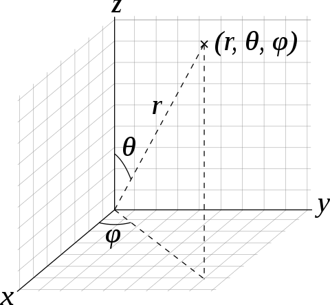
We can define the basis states of the spin as functions on the sphere, orthonormal with respect to the measure $sin(\theta)d\theta d\phi$. Here, $\theta$ is the polar angle (between $0$ and $\pi$) and $\phi$ is the azimuthal angle (between $0$ and $2\pi$).
$\phi_{j,m}(\theta, \phi) = \frac{1}{\sqrt{4\pi}}\sqrt{\begin{pmatrix} 2j \\ j+m \end{pmatrix}}cos(\frac{\theta}{2})^{j+m}sin(\frac{\theta}{2})^{j-m}e^{-i(j-m)\phi}$
In similar terms, we can define the coherent states, which have $2j$ stars at the point $(\theta, \phi)$:
$\mid \theta, \phi \rangle = \sum_{m=-j}^{j} \sqrt{\begin{pmatrix} 2j \\ j+m \end{pmatrix}}cos(\frac{\theta}{2})^{j+m}sin(\frac{\theta}{2})^{j-m}e^{i(j-m)\phi}\mid j, m\rangle$
We have: $\langle \theta, \phi \mid \theta, \phi \rangle = 1$ and $\int_{\phi=0}^{\phi=2\pi} \int_{\theta=0}^{\theta=\pi} \frac{sin(\theta)d\theta d\phi}{4\pi} \mid \theta, \phi \rangle \langle \theta, \phi \mid = I$.
We then consider:
$\langle j, m \mid \theta, \phi \rangle = \sqrt{\begin{pmatrix} 2j \\ j+m \end{pmatrix}}cos(\frac{\theta}{2})^{j+m}sin(\frac{\theta}{2})^{j-m}e^{i(j-m)\phi}$
So that:
$|\langle j, m \mid \theta, \phi \rangle|^{2} = \begin{pmatrix} 2j \\ j+m \end{pmatrix}cos^{2}(\frac{\theta}{2})^{j+m}sin^{2}(\frac{\theta}{2})^{j-m}$
Now recall the binomial distribution. We have $n$ trials, and there is a probability $p$ of success and a probability $1-p$ of failure in each trial. The question is: what is the probability of getting $k$ successes?
$Pr(k) = \begin{pmatrix}n \\ k \end{pmatrix}p^{k}(1-p)^{n-k}$
Why? To quote wikipedia: "$k$ successes occur with probability $p^{k}$ and $n − k$ failures occur with probability $(1 − p)^{n − k}$. However, the $k$ successes can occur anywhere among the $n$ trials, and there are ${\binom {n}{k}}$ different ways of distributing $k$ successes in a sequence of $n$ trials."
Suppose we have $n=2j$ trials, and $p_{win} = cos^{2}(\frac{\theta}{2})$ and $p_{loss} = 1 - p_{win} = sin^{2}(\frac{\theta}{2})$. We're interested in the probability of winning $k = j+m$ trials.
We then have $Pr(k) = \begin{pmatrix}2j \\ j+m \end{pmatrix}cos^{2}(\frac{\theta}{2})^{j+m}sin^{2}(\frac{\theta}{2})^{j-m} = |\langle j, m \mid \theta, \phi \rangle|^{2}$
In other words, $|\langle j, m \mid \theta, \phi \rangle|^{2}$, the probability of measuring a coherent state at $(\theta, \phi)$ to be in the basis state $\mid j, m\rangle$ is that same as the probability of winning $j+m$ out of $2j$ trials where the probability of winning a single trial is given by $cos^{2}(\frac{\theta}{2})$.
When $\theta=0$, $p_{win} = cos^{2}(0) = 1$. In other words, if our coherent state is at the north pole, we're certain to win. When $\theta=\pi$, $p_{win} = cos^{2}(\frac{\pi}{2}) = 0$, so that if our coherent state is at the south pole, we're certain to lose. At the equator, we have a 50/50 shot each time: $p_{win} = \frac{1}{2}$. (Recall we've quantized along the $Z$ axis.)
You might wonder how we obtain the above representation of a spin coherent state. Here's the sketch of a proof, again due to Gazeau.
We can represent a rotation of $\omega$ around an axis $(x, y, z)$ with: $e^{-i\omega(x\sigma_{X} + y\sigma_{Y} + z\sigma_{Z})}$.
Now recall that if we have some unit vector pointing to $(\theta, \phi)$ in spherical coordinates, then its expression in cartesian coordinates is: $(sin(\theta)cos(\phi), sin(\theta)sin(\phi), sin(\theta)cos(\theta))$.
We can consider a rotation that takes the point $(0,0,1)$ to that unit vector:
$e^{-i\theta(-sin(\phi)\sigma_{X} + cos(\phi)\sigma_{Y})}$.
Now if we define $\chi = -\frac{\theta}{2}e^{-i\phi}$, this can be rewritten: $e^{(\chi\sigma_{+} - \overline{\chi}\sigma_{-})}$.
The $\mid j, j \rangle$ state is the state with all the stars at the North Pole. Since a spin coherent state is defined by all the stars located at the same point, each spin coherent state can be obtained from rotating the $\mid j, j \rangle$ state.
$\mid \theta, \phi \rangle = e^{(\chi\sigma_{+} - \overline{\chi}\sigma_{-})}\mid j, j \rangle$, where again $\chi = -\frac{\theta}{2}e^{-i\phi}$.
Using the Baker-Campell-Hausdorff formula, one can finagle $e^{(\chi\sigma_{+} - \overline{\chi}\sigma_{-})}$ into the following form:
$e^{-\overline{z}\sigma_{+}}e^{ln(1+|z|^{2})\sigma_{Z}}e^{z\sigma_{-}} = e^{z\sigma_{-}}e^{-ln(1+|z|^{2})\sigma_{Z}}e^{-\overline{z}\sigma_{+}}$
Here, $z = - \frac{\overline{\chi}}{|\chi|} \frac{sin(|\chi|)}{cos(|\chi|)} = tan(\frac{\theta}{2})e^{i\phi}$, the stereographic projection from the South Pole.
We then have:
$\mid z \rangle = \mid \theta, \phi \rangle = e^{z\sigma_{-}}e^{-ln(1+|z|^{2})\sigma_{Z}}e^{-\overline{z}\sigma_{+}}\mid j, j \rangle$
But $e^{-\overline{z}\sigma_{+}}\mid j, j \rangle = \mid j, j \rangle$, since $\sigma_{+}$ gives the zero vector on $\mid j, j\rangle$ so that all but the first term (the identity) are irrelevant in the exponential series.
Then it turns out that: $e^{-ln(1+|z|^{2})\sigma_{Z}}\mid j, j \rangle = cos(\frac{\theta}{2})^{2j}\mid j, j \rangle$
This leaves us with $\mid \theta, \phi \rangle = cos(\frac{\theta}{2})^{2j}e^{z\sigma_{-}}\mid j, j \rangle$.
Working this out gives:
$\mid z \rangle = \mid \theta, \phi \rangle = \sum_{m=-j}^{j} \sqrt{\begin{pmatrix} 2j \\ j+m \end{pmatrix}}cos(\frac{\theta}{2})^{j+m}sin(\frac{\theta}{2})^{j-m}e^{i(j-m)\phi}\mid j, m\rangle$