Let's recap.
Our narrative has followed a particular thread: the generalization of the concept of number until it's adequate to describe the numbers which appear in physics.
We've organized things, perhaps arbitrarily, through the unfolding of a "dialectic."
A word on this choice may be in order. The idea of a dialectic goes back at least to the beginning of written philosophy, and really in the end is just the idea that through a "dialogue" you can get farther than you can with a "monologue." The point being that the results of a dialogue can't be totally anticipated beforehand.
Whereas monological philosophy proceeds by definitions and confines itself to what can be proven from those definitions, fixing a set of static concepts at the beginning, dialogic philosophy tracks how concepts play off each other and evolve, emphasizing how seemingly irreconcilable ideas can often be unified in surprising ways by appealing to new points of view. A monologue explains a concept; a dialectic tells a story about concepts.
It's not, however, a question of a dialogue always being better than a monologue. Rather, the dialectic is especially helpful when one isn't just delivering new or useful information, but instead, when there are many intellectual knots to untie, when there are many prejudices, preconcieved notions that need to be deconstructed before a new structure can be built. The original dialectician was Socrates, who never had some systematic theory of the world, but instead, stood in the Forum, challenging people by showing them the contradictions in the way they themselves used words.
On the other hand, if you take a philosophy class, the character most famously associated with a "dialectic" is the German idealist Hegel. A caricature of a Hegelian dialectic goes like this: First, you have a thesis. Then, the thesis calls into existence its antithesis. Finally, the thesis and antithesis are overcome by a synthesis, which resolves them together, but which couldn't have been anticipated by mere analysis of the thesis and antithesis, which are by definition irreconcilable in their own terms. A new cycle begins: the synthesis itself acts as a thesis, bringing forth an antithesis, etc. Thesis, antithesis, synthesis: they could be ideas, states of consciousness, material situations, designs of spirit--it's left open to interpretation.
Hegel famously used this device to try to retell human history as part of the dialectical unfolding of ideas in a cosmic spirit, whose intellectual development tracks the changes in the structure of the material world, and whose ultimate aim is absolute self-knowledge. In the next chapter of the history of philosophy, the young upstart Karl Marx turns Hegel on his head, applying dialectical reasoning to the material/social/economic affairs of different time periods, capitalism resolving the contradictions of feudal world, communism resolving the contradictions of capitalism, etc. After that intervention, the reputation of so-called "dialectical reasoning" has often been entangled with politics.
I personally think that mathematics benefits from a dialectical exposition. First of all, mathematics is often difficult to learn because it is so conceptually unified: where do you start? Mathematics is the true heaven of coincidences. Every idea is used and reused and resonates across different scales of the subject, and to grasp the importance of even simple things, one has had to scale mountains. Whenever one teaches, one has to chart one of many possible paths through the territory, and the question arises of how best to tell the story. Often, to proceed step by step makes it impossible to grasp the long arc; yet to elide over details allows misunderstanding to creep in.
On the other hand, things like Godel's theorems establish that sufficiently complicated formal mathematical systems can't coherently talk about themselves. They can only be analyzed from some higher vantange point. Furthermore, physics is always tugging mathematics by the hand, establishing empirical correspondences that couldn't have been deduced by pure analysis alone.
With all that in mind, I've tried to tell one possible story about the "dialectical unfolding of the concept of number," which is probably where Hegel's rather rigid concept of a dialectic is actually most applicable, in the end.
We began (1) by investigating our most basic idea of a "pebble," a "bit." We could place a pebble somewhere, and we could take it away. To communicate with a pebble, we had to agree on whether presence or absence would be significant. As much a theory of numbers, we began developing a theory of symbols, which can be placed, erased, symbols symbolizing symbols, etc, and which come with rules which are necessary to abide by so that communication via those symbols is reliable.
From (1), we asked: Why not place another pebble? And another, and another? And make a little pile of indistinguishable pebbles. And so we invented the counting numbers (2). To communicate with a counting number, we have to agree on what number we start counting from. So a pile of pebbles is like the contextualization of our original pebble: this pebble is actually the 4th pebble, if you've been keeping count, and to keep count is: to build up a little pile. So the pile is a contextualization of the pebble.
Then (3), we imagined iterating "counting" itself, counting "all at once," and so we invented addition, or combining piles. We had to have an inverse operation, and so we invented the negative numbers when it became clear that we had to be able to subtract past 0, and in this way achieved a synthesis: the "integers." To communicate with an integer, we have to agree on what is 0, and also which direction we're in, positive or negative.
Then (4), we imagined iterating addition to get multiplication, whose inverse is division. We thus discovered the rational numbers, or piles of "prime pebbles." We could now contextualize a pile of pebbles by specifying a rational number which translates between your units and my units, between our different ideas of "1". We also noticed that allowing division by 0 wraps the number line into a circle.
Then (5), we imagined iterating multiplication to get exponentiation, whose inverse is root-taking. We thus discovered the irrational numbers like the $\sqrt 2$, but also the complex numbers $a + b\sqrt{-1}$. We could thus rotate between two coordinate axes. And hidden inside, was a third axis, turning the plane into a sphere if we allow division by 0.
We saw how our numbers turned reflexive, leading us to reflect on the general theory of computation and its limitations. We observed that no single set of logical atoms which are powerful enough to axiomatize arithmetic can be both consistent and complete, able to prove all true theorems about itself, and indeed, one such undecidable theorem is the consistency of the formal system itself. In other to prove the consistency of such a logical system, one has to move to a larger, more powerful system, adding axioms, which leads to yet other undecidable truths, which can only be decided with yet more axioms. The point being that one can't start from a single set of axioms and rules for inference and imagine a machine trying out every possible rearrangement of symbols and thus proving all possible theorems. This suggests that conceptually, there can't be a single set of "master concepts" from which all concepts can be mechanically derived. Pure deduction can only take you so far. For example, you could spend all day thinking about the nature of probability in terms of probability theory and you'd never be able to derive the surprising ways that probabilities enter into our theory of physics.
Then (6), we began by considering an unordered "pile" of complex numbers, which we associated with points on the plane/sphere, and realized we could interpret them as the roots of a polynomial, giving us a yet higher order version of the idea of a "pile of pebbles": an equation. By the fundamental theorem of algebra, these unordered roots could be interpreted as a unique ordered sequence of coefficients up to a complex number. Out of the question of the solvability of equations, we extracted the theory of groups.
In (7), we emphasized that polynomials form a vector space. We realized we could interpret finite degree polynomials as "quantum states," specifically as the spin states of spin-$j$ particles, intepreting the roots of the polynomial as a constellation on the sphere, each root carrying a quantum of angular momentum $\frac{1}{2}$.
Vectors, however, are only defined up to a set of basis vectors. Hermitian matrices, which correspond to observables in quantum mechanics, automatically provide such basis sets via their eigenvectors. We've expanded our notion of a number to include a "matrix," finite or infinite, whose multiplication rule isn't commutative, and which can therefore furnish representations of symmetry groups, in particular, the unitary representations of quantum mechanics.
Indeed, linear algebra provides the theory of generalized "perspective switches," and we realized we could generalize our idea of perspective to that of an "experimental situation," by which a state is filtered probablistically into outcome states, the latter of which provide a complete basis for the Hilbert space of the state.
In (8), we considered "matrices of matrices": tensors. The tensor product is the way that quantum systems combine, and its properties lead to much of the quantum "magic."
In one of the great twists of all time, entanglement proves that any simple reductionism can't work in science. When particles get entangled, there is more information in the whole than in the parts. For example, in the antisymmetric state, two spin-$\frac{1}{2}$ particles are maximally uncertain with regard to their individual rotation axis, but their entanglement means that they must always point in the opposite direction. So that if one is measured to be $\uparrow$, the other one must be $\downarrow$ in any direction. Of course, through repeated experimentation on the two particles, one could precisely determine the quantum state of the whole, that it was in the antisymmetric state. But for each instance of the experiment, there is more information contained in the two particles together, in their "jointness," than can be extracted from the parts.
Continuing the spin theme, we realized that the symmetric tensor product of $2j$ spin-$\frac{1}{2}$ states also gives us a representation of a spin-$j$ state, where the "constellation" is encoded "holographically" in the entanglement between the spin-$\frac{1}{2}$'s. This itself was foreshadowed in the holistic relationship between the roots of a polynomial and its coefficients. Perhaps that's the twist: even if we have $2j$ spatially separate permutation symmetric spin-$\frac{1}{2}$'s, where the entangled whole is greater than the parts, from another point of view the same situation can be described as a simple juxtaposition: a product of roots, constellated on the sphere.
We discussed the theory of Clebsch-Gordan coefficients, and the idea that the tensor product of a bunch of spins could be decomposed into separate sectors with different $j$ values, turning the AND of the tensor product into the OR of a choice. And so we arrived at the theory of angular momentum conserving interactions with allusions to spin networks, which by the way, can be generalized to other types of interactions that conserve other quantities besides angular momentum. And we realized that angular momentum conserving vertices could be interpreted as the quantum polyhedra of loop quantum gravity, "atoms of space."
In (9), we discussed the quantum harmonic oscillator, a kind of twin to spin, the two being the simplest and arguably most fundamental quantum systems. Instead of interpreting the roots of a polynomial as living on the sphere (the classical phase space of a rotating object), we interpret the roots of the polynomial as living on the plane (interpreted as the classical phase space of a harmonic oscillator, the real axis being position and the imaginary axis being momentum). We discussed in this context coherent states, and coherent state quantization, which I poetically described as viewing quantum mechanics as an extension of classical mechanics that allows for negative definitions, the roots corresponding to multiple forbidden classical states. And we discussed the theory of the oscillator itself, full of indistinguishable, countable energy quanta, comparing the wave function representation to the polynomial representation.
We then graduated to second quantization: We imagined introducing a quantum harmonic oscillator to each degree of freedom of a first quantized quantum system, upgrading it to a theory of indistinguishable particles (fermionic or bosonic). As an example, we introduced two harmonic oscillators, corresponding to the $\uparrow$ and $\downarrow$ states of a spin-$\frac{1}{2}$ state. The total fixed number subspaces of this Hilbert space turned out to correspond to spin-$0$, spin-$\frac{1}{2}$, spin-$1$, $\dots$ Hilbert spaces, each of them indeed corresponding to a permutation symmetric tensor product of spin-$\frac{1}{2}$'s. And so we developed a representation capable of expressing a superposition of spins with different $j$ values, which was also a representation of the polarization of light, and in either case was a theory of indistinguishable particles. And we alluded how we could develop the representation theory of other groups using the same method, e.g. $SU(3)$, and how in quantum field theory, we're also dealing with the position/momentum states. We digressed on the relationship between spin and statistics, and the use of oscillators in the Berry-Robbins construction.
The punchline here is that all known actual particles are of this type, indistinguishable quanta of some quantum field, albeit more complicated.
Zooming out, we can think about any measurement, in some sense, as being reducible to the measurement of some number operator, which is counting the number of "particles" in that state. And so, we've come full circle, able to contextualize our pebbles as counting the number of quanta of some mode of a quantum field. Indeed, we could say that the world is conceptually made of "pebbles" insofar as we can use pebbles, appropriately contextualized, to represent it. And indeed, the particles in nature are indistinguishable just like pebbles in a pile.
But the story isn't over yet.
When one works with relativistic quantum field theory, a basic demand is that the vacuum state (with no particles) is Lorentz invariant. In other words, translated, rotated, boosted observers all agree on the vacuum state, indeed, on the idea of "what is a particle." This leads to Wigner's classification scheme based on mass and spin. The idea is that what we mean by a "particle" should be invariant, or the same, whether we rotate it, whether we translate it, whether we translate by it, whether we see it while moving at top speed, etc. In other words, we define a particle in terms of what we can do that leaves it the same, as something left invariant under the different perspectives we might have on it, in this case, inertial frames.
(Sidebar: today in the field of neural networks, people are starting to build networks which explictly respect the underlying group structure of some domain, the classic example being learning representations of images that are translation invariant using convolutional neural networks. The idea, of course, being that a neural network should be able to recognize the identity of something even if it's seen askew--and you can really help it along if you make sure its representation is invariant under some group.)
Now we won't go into the subtleties of relativistic quantum field theory here, how it necessarily leads to a theory of multiple particles, how one has to consider infinite numbers of possible interactions between particles, perhaps using Feyman diagrams or harder stuff, how one has to deal with renormalizing such infinities by considering how the different scales of a system relate to each other, how one can then consider the landscape of QFT's organized by scale, and how conformal field theories (which are scale invariant, like the Ising model at the critical temperature) are like landmarks in the space of all QFT's, and many such interesting things, not to mention the simple internal gauge symmetries that lead to the Standard Model. Someday we shall discuss all that perhaps, but for now, I want to make a more specific point: what is one set of particles from one point of view may be another set of particles from another point of view. In other words, the perspectival interplay doesn't end with the quantum field: rather, even what one regards as space, time and particle is relative to some observer's point of view.
For example, when one moves to quantum field theory in a curved space, one employs (not necessarily unitary) canonical transformations between perspectives. Famously, in the Unruh effect, while an inertial observer in the vacuum will measure 0 particles, an accelerated observer will measure a non-0 number of particles!
One can consider Bogoliubov transformations, which can turn any Hamiltonian quadratic in creation and annihilation operators into a simple oscillator Hamiltonian: $\sum_{i} a^{\dagger}a$, etc, and which can mediate between the perspectives of the inertial and accelerated observers. This same technique can be used in condensed matter to describe how in certain systems electrons pair up to rove around as meta-particles. So that: what is one set of particles from one point of view may be another set of particles from another point of view.
On another side of things, there is a general theorem that the simple oscillator picture of fields falls apart at some point: Haag's Theorem, which says that an interacting theory is not necessarily unitarily equivalent to a free theory: imagine photons and electrons so tightly interacting that they can't be treated as separate entities. You might not even be able to do a tensor decomposition on the Hilbert space!
We've had occasion to discuss "symplectic" geometry way back when we discussed the meaning of the complex inner product. The name symplectic is kind of a joke: it's a translation into Greek of the Latin word "complex." Symplectic geometry is related to the phase space of classical mechanics. There, things come in pairs: one always as some kind of "position" paired to a "momentum," even if the meanings of these things become somewhat abstract. Hence, a similarity to complex numbers, which have two parts, real and imaginary. And clearly, the relationship between "symplectic" and "complex" runs deep: we've seen how in the case of the oscillator, we can interpret the complex plane as the symplectic position/momentum plane of the classical oscillator!
The point is that "symplectic" or "canonical" transformations transform positions and momenta among themselves so that you end up with another set of positions and momenta, that perserves the duality between momentum and positions.
We can consider finite linear symplectic transformations, which correspond to even dimensional "symplectic matrices".
It's easy to generate a random $2n$ x $2n$ symplectic matrix. The dimensions have to be even since we have pairs of $p$'s and $q$'s. First, generate four random real $n$ x $n$ matrices. Then tensor each one respectively with $I, iX, iY, iZ$, where $X, Y, Z$ are the $2$ x $2$ Pauli's and $I$ is the $2$ x $2$ identity. Sum them all up, and then do the $QR$ decomposition into a unitary matrix $Q$ times an upper triangular matrix $R$. $Q$ is the desired symplectic matrix.
Such a matrix preserves the so-called "symplectic form." We'll take the symplectic form $\Omega$ to be, for example, in the $6$ x $6$ case:
$\begin{pmatrix} 0 & -1 & 0 & 0 & 0 & 0 \\ 1 & 0 & 0 & 0 & 0 & 0 \\ 0 & 0 & 0 & -1 & 0 & 0 \\ 0 & 0 & 1 & 0 & 0 & 0 \\ 0 & 0 & 0 & 0 & 0 & -1 \\ 0 & 0 & 0 & 0 & 1 & 0 \end{pmatrix}$
In other words, a block diagonal matrix with $\begin{pmatrix} 0 & -1 \\ 1 & 0 \end{pmatrix}$'s along the diagonal.
A symplectic matrix $M$ will perserve $\Omega$ in the following sense:
$\Omega = M^{T}\Omega M$
import qutip as qt
import numpy as np
import scipy

def random_symplectic(n):
    R = [qt.Qobj(np.random.randn(n, n)) for i in range(4)]
    M = sum([qt.tensor(R[i], O) for i, O in \
             enumerate([qt.identity(2), 1j*qt.sigmax(), \
                        1j*qt.sigmay(), 1j*qt.sigmaz()])])
    Q, R = np.linalg.qr(M.full())
    return qt.Qobj(Q)

def omega(n):
    O = np.array([[0, -1],[1, 0]])
    return qt.Qobj(scipy.linalg.block_diag(*[O]*n))

def test(S, W):
    F = M.trans()*W*M
    return np.isclose(F.full(), W.full()).all()

n = 2
W = omega(n)
M = random_symplectic(n)
print(test(M, W))
In the quantum case, we could use a symplectic matrix to transform position and momenta operators among themselves in such a way that preserves the commutation relations.
Indeed, given some $R = \begin{pmatrix} Q_{0} \\ P_{0} \\ Q_{1} \\ P_{1} \\ \vdots \end{pmatrix}$, you can think about $\Omega$ as: $\Omega_{i,j} = tr(i[R_{i}, R_{j}])$ Naturally, this won't work unless $Q$ and $P$ are infinite dimensional and satisfying the canonical commutation relation: $[Q, P] = i$.
Now, one could imagine transforming not the $P$'s and $Q$'s but the $a$'s and $a^{\dagger}$'s. In this case, we call the transformations "Bogoliubov transformations." As I've said, linear Bogoliubov transformations can diagonalize quadratic Hamiltonians, and were first employed in the study of condensed matter systems, where certain particles can "pair up" and become "quasiparticles," moving around in their own right. In other words, the notion of "what is a particle" can be shifted with such a transformation.
In quantum optics, one simple Bogoliubov transformation is the following: we have a matrix paramterized by $r$:
$\begin{pmatrix} cosh(r) & -sinh(r) \\ -sinh(r) & cosh(r) \end{pmatrix} \begin{pmatrix} a \\ a^{\dagger}\end{pmatrix} = \begin{pmatrix} b \\ b^{\dagger}\end{pmatrix}$
So that:
$b = a \ cosh(r) - a^{\dagger} \ sinh(r)$
$b^{\dagger} = a^{\dagger} \ cosh(r) - a \ sinh(r)$
This same transformation can be implemented with the "single mode squeezing operator":
$S = e^{ \frac{r(a^{2} - a^{\dagger2})} {2}}$
In general, we can have a complex parameter $z$ with:
$S = e^{ \frac{\overline{z}a^{2} - za^{\dagger2}}{2}}$
If $z = re^{i\theta}$:
$\begin{pmatrix} cosh(r) & -e^{i\theta}sinh(r) \\ -e^{-i\theta}sinh(r) & cosh(r) \end{pmatrix} \begin{pmatrix} a \\ a^{\dagger}\end{pmatrix} = \begin{pmatrix} b \\ b^{\dagger}\end{pmatrix}$
The squeezing operator is useful since we can act on states easily. For example, acting on the vacuum state $\mid 0 \rangle$, we get the "squeezed" vacuum. (Note the similarity to a coherent state.) Check out osc_coherent_picker.py and uncomment state = squeezed_coherent(s) to explore.
import qutip as qt
import numpy as np

n = 10
a = qt.destroy(n)
r = np.random.rand()

S = (r*(a*a - a.dag()*a.dag())/2).expm()
a2, adag2 = S.dag()*a*S, S.dag()*a.dag()*S

vac = qt.basis(n, 0)
squeezed_vac = S.dag()*vac

print("N on vac: %.4f" % qt.expect(a.dag()*a, vac))
print("N2 on vac: %.4f" % qt.expect(a2.dag()*a2, vac))
print("-")
print("N on squeezed vac: %.4f" % qt.expect(a.dag()*a, squeezed_vac))
print("N2 on squeezed vac: %.4f" % qt.expect(a2.dag()*a2, squeezed_vac))
We can also consider "two-mode squeezing."
Given some parameter $r$, we have a Bogoliubov transformation:
$\begin{pmatrix} cosh(r) & 0 & 0 & sinh(r) \\ 0 & cosh(r) & sinh(r) & 0 \\ 0 & sinh(r) & cosh(r) & 0 \\ sinh(r) & 0 & 0 & cosh(r) \end{pmatrix} \begin{pmatrix} a_{0} \\ a_{1} \\ a_{0}^{\dagger} \\ a_{1}^{\dagger} \end{pmatrix}$
The two mode squeezing operator is:
$S = e^{r(a_{0}a_{1} - a_{0}^{\dagger}a_{1}^{\dagger})}$
import qutip as qt
import numpy as np

n = 2
a = [qt.tensor(qt.destroy(n), qt.identity(n)),\
     qt.tensor(qt.identity(n), qt.destroy(n))]
r = np.random.rand()
O = a + [a_.dag() for a_ in a]

S = (r*(a[0]*a[1] - a[0].dag()*a[1].dag())).expm()
O2 = [S.dag()*o*S for o in O]

vac = qt.basis(n**2, 0)
vac.dims = [[n, n],[1,1]]
squeezed_vac = S.dag()*vac

print("Na on vac: %.4f" % qt.expect(a[0].dag()*a[0], vac))
print("Nb on vac: %.4f" % qt.expect(a[1].dag()*a[1], vac))

print("N2a on vac: %.4f" % qt.expect(O2[0].dag()*O2[0], vac))
print("N2b on vac: %.4f" % qt.expect(O2[1].dag()*O2[1], vac))

print("-")

print("Na on squeezed vac: %.4f" % qt.expect(a[0].dag()*a[0], squeezed_vac))
print("Nb on squeezed vac: %.4f" % qt.expect(a[1].dag()*a[1], squeezed_vac))

print("N2a on squeezed vac: %.4f" % qt.expect(O2[0].dag()*O2[0], squeezed_vac))
print("N2b on squeezed vac: %.4f" % qt.expect(O2[1].dag()*O2[1], squeezed_vac))
Also check out tm_squeeze_picker.py. You can drag a point around the complex plane to pick the squeezing parameter and visualize the two mode squeezed state in terms of the position amplitudes of the two oscillators in the plane and also its decomposition into spins.
Another application of the "two mode squeezed vacuum" is the analysis of the Unruh effect.
An inertial observer is hanging around Minkowski space, not detecting any particles of some scalar field. In other words, the scalar field is in its vacuum state, without any particles. All inertial observers agree on this vacuum state, and hence: on what is meant by a particle. The vacuum state is "Lorentz invariant." But what about an accelerated observer? For example, a constantly accelerated observer. The prediction of Unruh is that such an observer would detect particles: in other words, the scalar field would not be in its vacuum state from that perspective, in fact, it would be in a "squeezed vacuum."
One can describe the situation with respect to the constantly accelerating observer with "Rindler coordinates."
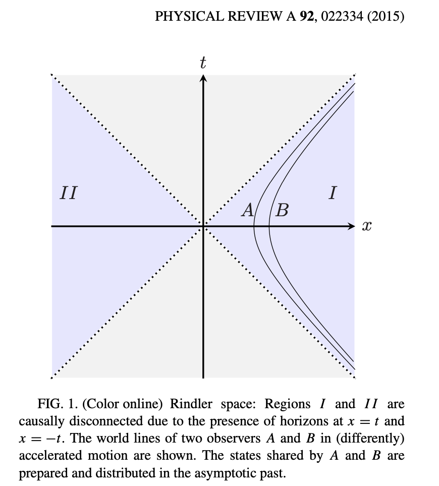
The idea is that because of their constant acceleration, the world of the accelerated observer is divided into two: they're confined to the $I$ region. There is a kind of "horizon" to their experience.
Following this paper, suppose we consider a real massless scalar quantum field in 1+1 dimensions. It's "modes" correspond to solutions of the Klein-Gordon equation:
$\frac{1}{c^2} \frac{\partial^2}{\partial t^2} \psi - \frac{\partial^{2}}{\partial x^{2}} \psi + \frac{m^2 c^2}{\hbar^2} \psi = 0$
For a given momentum mode of the scalar field $k$, in Minkowski coordinates:
$m_{k}(x, t) = \frac{1}{\sqrt{4\pi|k|}}e^{i(kx - |k|t)}$
We have:
The energy operator $E = i\frac{\partial}{\partial t}$.
The boost operator $K = i(x\frac{\partial}{\partial t} + t\frac{\partial}{\partial x})$.
We, however, could also adopt Rindler coordinates, where $a$ is the acceleration.
$t = \frac{1}{a} e^{a\chi} sinh(a\tau)$
$x = \frac{1}{a} e^{a\chi} cosh(a\tau)$
In these coordinates, the boost operator is $K = \frac{i}{a}\frac{\partial}{\partial\tau}$, and the Hamiltonian is given by $aK = i\frac{\partial}{\partial\tau}$.
But there are actually two coordinate patches, for $I$ and $II$.
$t = \frac{1}{a} e^{a\chi^{\prime}} sinh(a\tau^{\prime})$
$x = -\frac{1}{a} e^{a\chi^{\prime}} cosh(a\tau^{\prime})$
In this patch, the boost operator $K = -\frac{i}{a}\frac{\partial}{\partial\tau^{\prime}}$.
Let's consider two Rindler modes, one in each patch:
$r_{I, k}(\chi, \tau) = \frac{1}{\sqrt{4\pi|k|}}e^{i(k\chi - |k|\tau)}$
$r_{II, k}(\chi^{\prime}, \tau^{\prime}) = \frac{1}{\sqrt{4\pi|k|}}e^{i(-k\chi^{\prime} - |k|\tau^{\prime})}$
And then let's consider the creation and annihilation operators of these two modes: $\rho_{I}$ and $\rho_{II}$. In other words, $\rho_{I}, \rho_{I}^{\dagger}$ and $\rho_{II}, \rho_{II}^{\dagger}$.
We've supposed our accelerating observer is moving with acceleration $a$.
We form the two mode squeezing operator:
$ S = e^{ r_{k} (\rho_{I}\rho_{II} - \rho_{I}^{\dagger}\rho_{II}^{\dagger})}$
Where $r_{k} = arctan(e^{-\frac{\pi|k|}{a}})$.
If $\mid 0 \rangle_{I}\mid 0 \rangle_{II}$ is the Rindler vacuum, then: $ S\mid 0 \rangle_{I}\mid 0 \rangle_{II} = \mid 0 \rangle_{M}$ gives the Minkowski vacuum. In other words, what is the Minkowski vacuum for the inertial observer is an entangled state across $I$ and and $II$ (with particles) for the Rindler observer, who in any case is confined to the region $I$, and so has to partial trace over $II$. It's as if by accelerating, the observer has traded spatial connectivity for entanglement!
import qutip as qt
import numpy as np

n = 4
rI = qt.tensor(qt.destroy(n), qt.identity(n))
rII = qt.tensor(qt.identity(n), qt.destroy(n))
r_vac = qt.tensor(qt.basis(n,0), qt.basis(n,0))

a = 20000*np.random.rand()
k = 100*np.random.rand()
r = np.arctan(np.exp(-np.pi*abs(k)/a))
SQ = (r*(rI*rII - rI.dag()*rII.dag())).expm()
m_vac = SQ*r_vac
#m_vac = qt.tensor(qt.rand_ket(n), qt.rand_ket(n))

m = qt.destroy(n**2)
m.dims = [[n,n], [n,n]]
m = SQ*m*SQ.dag()

print("momentum: %.4f, acceleration: %.4f" % (k, a))
print("N_rI on rindler vac: %.4f" % qt.expect(rI.dag()*rI, r_vac))
print("N_rII on rindler vac: %.4f" % qt.expect(rII.dag()*rII, r_vac))
print("N_m on rindler vac: %.4f" % qt.expect(m.dag()*m, r_vac))
print("-")
print("N_rI on minkowski vac: %.4f" % qt.expect(rI.dag()*rI, m_vac))
print("N_rII on minkoswki vac: %.4f" % qt.expect(rII.dag()*rII, m_vac))
print("N_m on minkowski vac: %.4f" % qt.expect(m.dag()*m, m_vac))

print()
print(m_vac.ptrace(0), qt.entropy_vn(m_vac.ptrace(0)))
print(m_vac.ptrace(1), qt.entropy_vn(m_vac.ptrace(1)))
There is an inverse relationship: if an inertial observer would measure no particles, then an accelerated observer would measure some particles. And if an accelerated observer would measure no particles, then an inertial observer would measure some. Indeed, if the accelerated observer were to measure a particle, this would naturally disentangle the two halves, leading to the appearence of particles from the inertial perspective.
Finally, similar arguments (comparing the mode decomposition of a field from two different perspectives) yield the famous Hawking radiation. In the Unruh case, a stationary observer observes no particles, but an accelerated observer does (and indeed, the two disconnected halves of Rindler space are entangled.) In the Hawking case, a stationary observer far from the black hole observes particles popping out of the curved spacetime, entangled across the event horizon of the black hole, which eventually causes the black hole to radiate away its insides.
In the Unruh case, the accelerated observer would detect a thermal spectrum of particles with temperature $T = \frac{\hbar a}{2\pi c k_{b}}$. In the second case, the stationary observer would detect a thermal spectrum of particles from the black hole with temperature $T = \frac{\hbar \kappa}{2\pi c k_{b}}$, where $\kappa$ is the surface gravity. (See discussion on quora). By the equivalence principle, they are basically the same thing.
(For an accessible but more detailed account of the Unruh effect see here.
The observer dependence of space, time, and particle reaches its culmination in our current, not entirely worked out theories of quantum gravity.
In holographic theory, one has, for example, a conformal field theory on the boundary of some space (like on the surface of the sphere) being from another point of view a gravitational theory in the interior of that space (like in the interior of the sphere), usually an anti-DeSitter space, one with negative curvature, so that signals going off to infinity, return in finite time--just like the inside of a black hole.
Indeed, this was the initial motivation: one wants to regard the seemingly inaccessible quantum state of the interior of the black hole (including the things that fall into it) as being, from another perspective, the quantum state that lives on a surface, the event horizon (and also the Hawking radiation). In these models, there is an interesting connection between phenomena that extend across large scales of the boundary and phenomena that occur deep in the interior of bulk of the "emergent spacetime."
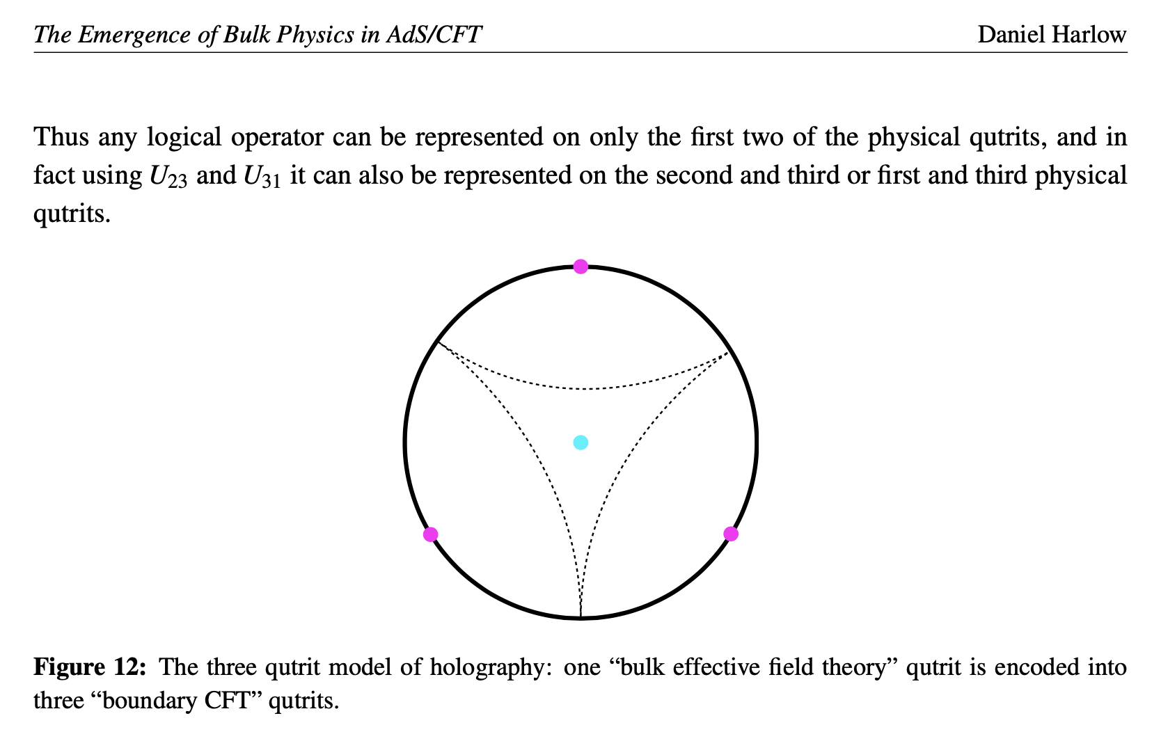
We've already had occasion to discuss black holes in the context of our simple wormhole models, to which we shall shortly return at long last. Here, let's confine ourselves to looking at perhaps the simplest model of "holography": the three-qutrit error correcting code.
The basic idea is that we can encode the state of a single qutrit (or spin-$1$ state) in the entanglement between three qutrits using the following map:
$\mid 0 \rangle \rightarrow \frac{1}{\sqrt{3}} \big{(} \mid 000 \rangle + \mid 111 \rangle + \mid 222 \rangle \big{)}$
$\mid 1 \rangle \rightarrow \frac{1}{\sqrt{3}} \big{(} \mid 012 \rangle + \mid 120 \rangle + \mid 201 \rangle \big{)}$
$\mid 2 \rangle \rightarrow \frac{1}{\sqrt{3}} \big{(} \mid 021 \rangle + \mid 102 \rangle + \mid 210 \rangle \big{)}$
Here, $\mid 0 \rangle, \mid 1 \rangle, \mid 2 \rangle$ are the three basis states of the qutit.
Using this correspondence, we can create a linear map $T$ which can upgrade a qutrit into a state of the three, such that $T^{\dagger}$ downgrades three to one, and $T^{\dagger}T = I$. (By the way, as a tensor consisting of four qutrits, $T$ is a "perfect" tensor in that any bipartition of its indices leads to an isometry.)
import qutip as qt
import numpy as np

def make(s, n=3):
    return qt.tensor(*[qt.basis(n, int(s[i])) for i in range(len(s))])

zero = (make("000") + make("111") + make("222"))/np.sqrt(3)
one = (make("012") + make("120") + make("201"))/np.sqrt(3)
two = (make("021") + make("102") + make("210"))/np.sqrt(3)

one_three = qt.Qobj(np.array([zero.full().T[0],\
                              one.full().T[0],\
                              two.full().T[0]]).T)
one_three.dims = [[3,3,3], [3]]

qutrit = qt.rand_ket(3)
three_qutrits = one_three*qutrit

X, Y, Z = qt.jmat(1, 'x'), qt.jmat(1, 'y'), qt.jmat(1, 'z')
X_, Y_, Z_ = one_three*X*one_three.dag(), one_three*Y*one_three.dag(), one_three*Z*one_three.dag()

xyz1 = np.array([qt.expect(X, qutrit), qt.expect(Y, qutrit), qt.expect(Z, qutrit)])
xyz2 = np.array([qt.expect(X_, three_qutrits), qt.expect(Y_, three_qutrits), qt.expect(Z_, three_qutrits)])

print("xyz on original qutrit:")
print(xyz1)
print("xyz on encoded qutrit with upgraded ops:")
print(xyz2)

one_three.dag()*one_three
Now here's the fascinating thing, and what makes this an "error correcting code": we can recover the state of the original "logical" qutrit from any two of three "physical" qutrits.
Define $\chi = \frac{1}{\sqrt{3}} \big{(} \mid 00 \rangle + \mid 11 \rangle + \mid 22 \rangle \big{)}$.
And also a unitary $U$ which acts in the following way:
$\mid 00 \rangle \rightarrow \mid 00 \rangle$
$\mid 11 \rangle \rightarrow \mid 20 \rangle$
$\mid 22 \rangle \rightarrow \mid 10 \rangle$
$\mid 01 \rangle \rightarrow \mid 11 \rangle$
$\mid 12 \rangle \rightarrow \mid 01 \rangle$
$\mid 20 \rangle \rightarrow \mid 21 \rangle$
$\mid 02 \rangle \rightarrow \mid 22 \rangle$
$\mid 10 \rangle \rightarrow \mid 12 \rangle$
$\mid 21 \rangle \rightarrow \mid 02 \rangle$
Define $U_{1,2} = U \otimes I_{3}$, in other words, $U$ acting on the first two physical qutrits.
Similarly, $U_{2,3} = I_{3} \otimes U$, which acts on the last two physical qutrits.
And finally: $U_{3,1}$, which acts on the first and third, which you can get from $U \otimes I_{3}$ by permuting $(0,1,2) \rightarrow (1,2,0)$.
Suppose we have a logical qutrit $\mid \phi \rangle$ that we want to encode it in a state $\mid \widetilde{\phi} \rangle$ of the three physical qutrits. It turns out we can use any of these three unitaries to do the job, in conjuction with the $\mid \chi \rangle$ state.
$\mid \widetilde{\phi} \rangle = U_{1,2}(\mid \phi \rangle_{1} \otimes \mid \chi \rangle_{2,3}) = U_{2,3}(\mid \phi \rangle_{2} \otimes \mid \chi \rangle_{1,3}) = U_{3,1}(\mid \phi \rangle_{3} \otimes \mid \chi \rangle_{1,2}) $
Inversely, suppose we lose track of one of the physical qutrits, say the third. We can recover the logical qutrit with:
$U_{1,2}^{\dagger}\mid \widetilde{\phi} \rangle = \mid \phi \rangle_{1} \otimes \mid \chi \rangle_{2,3}$
chi = (make("00") + make("11") + make("22"))/np.sqrt(3)
UP = make("00")*make("00").dag() +\
     make("20")*make("11").dag() +\
     make("10")*make("22").dag() +\
     make("11")*make("01").dag() +\
     make("01")*make("12").dag() +\
     make("21")*make("20").dag() +\
     make("22")*make("02").dag() +\
     make("12")*make("10").dag() +\
     make("02")*make("21").dag()
UP_12 = qt.tensor(UP, qt.identity(3))
UP_23 = qt.tensor(qt.identity(3), UP)
UP_31 = qt.tensor(UP, qt.identity(3)).permute((1,2,0))

dm = qutrit*qutrit.dag()
encoded1 = UP_12*qt.tensor(qutrit, chi)
encoded2 = UP_23*qt.tensor_swap(qt.tensor(qutrit, chi), (0,1))
encoded3 = UP_31*qt.tensor(chi, qutrit)
print(encoded1.full().all() == encoded2.full().all() == encoded3.full().all() == three_qutrits.full().all())

qutrit_1 = one_three.dag()*encoded1
qutrit_2 = one_three.dag()*encoded2
qutrit_3 = one_three.dag()*encoded3
print(qutrit_1.full().all() == qutrit_2.full().all() == qutrit_3.full().all() == qutrit.full().all())

lost_third1 = encoded1.ptrace((0,1))
recovered1 = (UP.dag()*lost_third1*UP).ptrace(0)

lost_third2 = encoded1.ptrace((0,2))
UP_ = qt.tensor_swap(UP, (0,1))
recovered2 = (UP_.dag()*lost_third2*UP_).ptrace(0)

lost_third3 = encoded1.ptrace((1,2))
recovered3 = (UP.dag()*lost_third3*UP).ptrace(0)

print(recovered1.full().all() == recovered2.full().all() == recovered3.full().all() == dm.full().all())
For more information see here.
Calculating the mutual information between each physical qubit and the other two shows that they follow the "Ryu-Takayanagi formula": $2 ln(3)$. In this context, we can interpret this as: the mutual information between a boundary region $A$ and its complement $\overline{A}$ is given by twice the area of the minimal surface in the bulk. We can see that the area of the latter is just the entanglement entropy of any of the three qutrits.
print(qt.entropy_vn(three_qutrits.ptrace(0)))
print(qt.entropy_vn(three_qutrits.ptrace(0)))
print(qt.entropy_vn(three_qutrits.ptrace(0)))
print(np.log(3))

print("-")
print(qt.entropy_mutual(three_qutrits*three_qutrits.dag(), 0, (1,2)))
print(qt.entropy_mutual(three_qutrits*three_qutrits.dag(), 1, (0,2)))
print(qt.entropy_mutual(three_qutrits*three_qutrits.dag(), 2, (0,1)))

print(2*np.log(3))
Finally, we can consider iterating the construction to build up a toy model of a whole holographic spacetime:
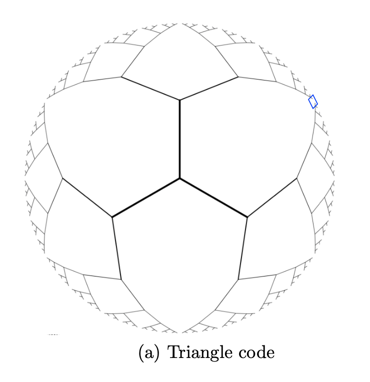
We can consider other such codes, and all sorts of "tensor networks," ways of hooking these maps into each other so that in some way the "bulk" is encoded in the entanglement between the states on the "boundary."
If this is supposed to model a black hole, we are confronted by two perspectives: on the one hand, if you stay outside the black hole, you deal with the boundary state and its radiating particles, and can mess with the interior state by acting at appropriate scales across the boundary. But, of course, you can access the interior in another way: simply by freely falling in. How the quantum system manifests itself as space, time, and particle depends on your state of motion.