Once upon a time, we started with a single pebble, and called it an "atom." We graduated to a "pile of pebbles," each pebble within a pile treated as identical, fungible. Even if the actual pebbles we might use to represent a pile are irregular in some respect, what we meant by "grouping them into a pile" was that insofar as they were in the pile, the pebbles were to be regarded as "indistinguishable" from each other, considered only insofar as they contributed to the "number of pebbles." And so we invented the counting numbers.
We then ascended the dialectical ladder, from counting numbers to integers to rationals to complex numbers to polynomials and at last to tensors, the latter corresponding the multiple joint perspectives of entangled quantum systems.
We're now going to consider "piles" of a yet higher-order sort, piles of identical quantum systems, piles which can keep track of a variable number of quantum systems, as indistinguishable as the "1"'s in a counting number. The mathematical structure we're looking for is essentially that of a "quantum field," although to call it a "field" is to emphasize one application of the structure, as we'll see. The general process of moving from ordinary quantum mechanics to a quantum mechanics of a variable number of indistinguishable "particles" is called "second quantization."
But to understand that, we first need to become familiar with the quantum harmonic oscillator. Then we can discuss perhaps the simplest example of second quantization, the oscillator representation of spin, also known as the "Jordan-Schwinger" representation. Since we already know so about spin states, we are already half-way there!
A review of the 1-dimensional quantum harmonic oscillator:
It's Hamiltonian is basically: $H = \frac{1}{2}(P^{2} + Q^{2})$, where $P$ is the momentum operator, whose eigenstates are states of definite momentum, and $Q$ is the position operator, whose eigenstates are states of definite position. These two operators are related to each other via the Fourier transform.
One great thing to do is define the creation and annihilation operators:
$a = \frac{1}{\sqrt 2} (Q + iP)$
$a^{\dagger} = \frac{1}{\sqrt 2} (Q - iP)$
So that: $Q = \frac{1}{\sqrt 2} (a^{\dagger} + a)$ and $P = \frac{1}{\sqrt 2} (a^{\dagger} - a)$.
Note that $[Q, P] = QP - PQ = i$. This is the Heisenberg uncertainty principle. And one thing it implies is that not only are $P$ and $Q$ not simultaneous measureable, but also, they can't be represented by any finite dimensional matrices, but only by "infinite" matrices. We'll see what this means.
Now what's nice about the creation and annihilation operators is that you can interpret them as adding or subtracting a "quantum" from the oscillator, kicking it up to a higher or lower "number" state (each of which has a higher or lower energy). These "number" states form a basis for the states of the oscillator, just as the position (or momentum) eigenstates do. To wit, if you can get the $\mid 0 \rangle$ quantum state, the ground state of the oscillator, then you can get all the other states, $\mid 1 \rangle, \mid 2 \rangle, \mid 3 \rangle, \ldots$ by repeated action of the creation operator.
The number operator, which counts the number of quanta, is $N = a^{\dagger}a$, and the hamiltonian can be rewritten $H = N + \frac{1}{2}$.
Notice:
$ N = \frac{1}{\sqrt 2}(Q - iP)\frac{1}{\sqrt 2}(Q + iP)$
$= \frac{1}{2}(Q^{2} + iQP - iPQ + P^{2}) $ $= \frac{1}{2}(Q^{2} + i(QP - PQ) + P^{2})$.
But $QP - PQ = i$, so we get $ N = \frac{1}{2}(P^{2} + Q^{2}) + -\frac{1}{2} = H - \frac{1}{2}$.
So $H = N + \frac{1}{2}$.
Already we can see that at least one way of thinking about a quantum harmonic oscillator is as a little guy that "counts quanta."
We should give a few words on the formalism of position and momentum wave functions, since hitherto we've only worked with finite dimensional Hilbert spaces.
A position wave function $\psi(x)$ is a function from the real numbers to the complex numbers, which is square integrable, and so can be interpreted as an "infinite dimensional vector." We have:
$Q\mid x \rangle = x\mid x \rangle$
$\langle x \mid x' \rangle = \delta(x - x')$
$\int \mid x \rangle \langle x \mid dx = I$
You can think of $\psi(x)$ as $\langle x \mid \psi \rangle$, where $x$ is a "Dirac delta" that spikes at position $x$. (There are some subleties here: because the deltas have infinite norm, they aren't technically vectors in the Hilbert space. One consequence is that to actually calculate legitimate probabilities, you need to integrate over some finite interval.)
You can take the Fourier transform of $\psi(x)$ to get $\psi(p)$, the momentum wave function. Similarly, you can use Dirac deltas that spike at momentum $p$, etc.
$P \mid p \rangle = p\mid p \rangle$
$\langle p \mid p' \rangle = \delta(p - p')$
$\int \mid p \rangle \langle p \mid dp = I$
By the nature of Fourier duality, a spike in position means an “oscillation” across momentum space. A spike in momentum means a “oscillation” across position space. For example, $\psi_{p}(x) = Ce^{ipx}$ where $C$ is a constant.
$\langle x \mid p \rangle = e^{ipx} $
$\langle p \mid x \rangle = e^{-ipx} $
$ \psi(x) = \int e^{ipx}\psi(p) dp = \int \langle x \mid p \rangle \langle p \mid \psi \rangle dp$
$ \psi(p) = \int e^{-ipx}\psi(x) dx = \int \langle p \mid x \rangle \langle x \mid \psi \rangle dx$
Given that we're working with infinite dimensional vector spaces, we have to treat the inner product as an integral, an infinite sum. In other words:
$\langle \phi \mid \psi \rangle = \int_{-\infty}^{+\infty} \phi(x)^{*}\psi(x) dx$, where the $*$ means take the complex conjugate.
Square summable means that $|\psi(x)|^{2} = \int_{-\infty}^{+\infty} \psi(x)^{*}\psi(x) dx$ converges to a real number (and so can be normalized to 1), and thus really can think of our wave function as being an vector in infinite dimensional space.
We recall that $Q\psi(x) = x\psi(x)$, that the position operator acts on a position wave function like multiplication by x, and $P\psi(x) = -i\frac{d}{dx}\psi(x)$, that the momentum operator acts like (multiplication by $-i$ and) differentiation. This was one of the initial insights of quantum mechanics: the so-called canonical quantization, promoting the classical variables $q$ and $p$ to linear operators $Q$ and $P$.
With this set of correspondences, we consider the time dependent Schrodinger equation for the harmonic oscillator.
$H\psi(x, t) = i\frac{d\psi(x, t)}{dt}$
$\frac{1}{2}(P^{2} + Q^{2})\psi(x, t) = i\frac{d\psi(x, t)}{dt}$
$\frac{1}{2}(-\frac{d^{2}}{dx^{2}} + x^{2})\psi(x, t) = i\frac{d\psi(x, t)}{dt}$
$ -\frac{1}{2}\frac{d^{2}\psi(x, t)}{dx^{2}} + \frac{1}{2}x^{2}\psi(x, t) = i\frac{d\psi(x, t)}{dt}$.
In terms of the time independent Schrodinger equation:
$ -\frac{1}{2}\frac{d^{2}\psi(x)}{dx^{2}} + \frac{1}{2}x^{2}\psi(x) - e\psi(x) = 0$, where $e$ is the eigenvalue corresponding to a given energy level.
There is a whole beautiful theory of these differential equations and how to solve them, and one finds that its infinitude of solutions are proportional to the Hermite polynomials. But actually there are some tricks we can use without actually solving the equations directly.
For example, we know that we want the annihilation operator to annihilate the ground state, which is also the 0 number state.
$a \psi_{0}(x) = 0$
$\frac{1}{\sqrt 2} (x + \frac{d}{dx})\psi_{0}(x) = 0 $
$x\psi_{0}(x) + \frac{d}{dx}\psi_{0}(x) = 0 $
A solution is given by:
$ \psi_{0}(x) = e^{-\frac{x^{2}}{2}}$
Which we can confirm:
$ \frac{d}{dx}\psi_{0}(x) = -xe^{-\frac{x^{2}}{2}}$
$ xe^{-\frac{x^{2}}{2}} -xe^{-\frac{x^{2}}{2}} = 0 $
Since $\int_{-\infty}^{+\infty} \psi(x)^{*}\psi(x) dx = \int_{-\infty}^{+\infty} e^{-x^{2}} dx = \sqrt{\pi}$, we should really use $\psi_{0}(x) = \pi^{\frac{1}{4}}e^{-\frac{x^{2}}{2}}$, but let's not get bogged down.
This function $\psi_{0}(x) = e^{-\frac{x^{2}}{2}}$ is interesting. It's a Gaussian, and it's invariant under the Fourier transform.
$\frac{1}{\sqrt{2\pi}} \int_{-\infty}^{\infty} e^{ipx}e^{-\frac{x^{2}}{2}}dx = e^{-\frac{p^{2}}{2}}$.
In other words, it represents the best compromise you can get between knowing both position and momentum given the Heisenberg uncertainty relations.
But is $\psi_{0}(x)$ really an eigenstate of $H$? Consider:
$H \psi_{0}(x) = (a^{\dagger}a + \frac{1}{2})\psi_{0}(x) = a^{\dagger}a\psi_{0}(x) + \frac{1}{2}\psi_{0}(x)$.
But we know that $a\psi_{0}(x)= 0$, so $H \psi_{0}(x) = \frac{1}{2}\psi_{0}(x)$.
Thus, $\psi_{0}(x)$ is an eigenvector of the harmonic oscillator hamiltonian: $H$ acts on $\psi_{0}(x)$ by multiplication by a scalar eigenvalue, in this case $\frac{1}{2}$. Since the annihilator annihilates it, we know that $\psi_{0}(x)$ is the lowest eigenvector of $N$ (and $H$), and we can get all the rest of the number states via the creation operator, just like climbing a ladder: indeed, they're known as ladder operators.
$\psi_{n}(x) = \frac{(a^{\dagger})^{n}}{\sqrt{n!}}\psi_{0}(x)$
This set of set of states $\psi_{n}(x)$ form a countable basis for our quantum harmonic oscillator. In other words, we can express any state $\phi(x)$ as an infinite series in the number states:
$\phi(x) = \sum_{n=0}^{\infty} c_{n}\psi_{n}(x)$, where:
$c_{n} = \frac{\psi_{n} \cdot \phi}{\psi_{n} \cdot \psi_{n}} = \frac{\int \psi_{n}^{*}(x)\phi(x)dx}{\int \psi_{n}^{*}(x)\psi_{n}(x)dx}$.
In other words, the projection of the function $\phi(x)$ onto the number state $\psi_{n}$, just like in the finite dimensional case, gives the coordinate in that "direction."
We can compare this to the case of breaking down sound waves into their harmonics.
If we have a real, continuous, periodic function $f(x)$ defined over the interval $r$ to $s$, we can write it as a Fourier series:
$ f(x) = a_{0}C_{0}(x) + \sum_{n=1}^{\infty} \Big{(} a_{n}C_{n}(x) + b_{n}S_{n}(x) \Big{)} $.
Here: $C_{0}(x) = 1$, $C_{n}(x) = cos(\frac{2\pi n x}{T})$, and $S_{n}(x) = sin(\frac{2\pi n x}{T})$, where $T$ is the period, and $n \in 1,2,3,\dots$.
$a_{0} = \frac{C_{0} \cdot f}{C_{0} \cdot C_{0}} = \frac{\int_{r}^{s} C_{0}(x)f(x) dx }{\int_{r}^{s} C_{0}(x)C_{0}(x) dx }$
$a_{n} = \frac{C_{n} \cdot f}{C_{n} \cdot C_{n}} = \frac{\int_{r}^{s} C_{n}(x)f(x) dx }{\int_{r}^{s} C_{n}(x)C_{n}(x) dx }$
$b_{n} = \frac{S_{n} \cdot f}{S_{n} \cdot S_{n}} = \frac{\int_{r}^{s} S_{0}(x)f(x) dx }{\int_{r}^{s} S_{n}(x)S_{n}(x) dx }$
This works because sines (and cosines) of different integer $n$ values are orthogonal, and so these functions can be treated as separate "directions" in infinite dimensional space.
Note that there are many ways of representing a function as an infinite series, often with different inner products, given by different measures.
Returing to the oscillator, let's prove that the number operator $N = a^{\dagger}a$ actually does count the number of quanta.
First, we consider the eigenvalue equation for $N$:
$N\psi_{n} = n\psi_{n}$
In other words, on a state of definite number, the number operator acts by multiplication by $n$, the number.
Let's consider acting with $N$ after we've raised the number by one: $Na^{\dagger}\psi_{n}$.
To evaluate this, first we note that:
$[a, a^{\dagger}] = aa^{\dagger} - a^{\dagger}a = \frac{1}{\sqrt 2} (Q + iP)\frac{1}{\sqrt 2} (Q - iP) - \frac{1}{\sqrt 2} (Q - iP)\frac{1}{\sqrt 2} (Q + iP)$
$ = \frac{1}{2} (Q^{2} -iQP +iPQ + P^2 - Q^{2} - iQP + iPQ - P^{2})$
$ = \frac{1}{2} (2iPQ - 2iQP)$
$ = i[P, Q] = -i[Q,P] = 1$
We then note that:
$[N, a^{\dagger}] = Na^{\dagger} - a^{\dagger}N = a^{\dagger}aa^{\dagger} - a^{\dagger}a^{\dagger}a = a^{\dagger}(aa^{\dagger} - a^{\dagger}a) = a^{\dagger}[a, a^{\dagger}] = a^{\dagger}$.
If $Na^{\dagger} - a^{\dagger}N = a^{\dagger}$, then $Na^{\dagger} = a^{\dagger}N + a^{\dagger}$.
So we can rewrite $Na^{\dagger}\psi_{n}$ as: $(a^{\dagger}N + a^\dagger)\psi_{n} = a^{\dagger}N\psi_{n} + a^\dagger\psi_{n}$.
But by the eigenvalue equation, this is: $na^{\dagger}\psi_{n} + a^\dagger\psi_{n} = (n+1)a^{\dagger}\psi_{n}$.
In short, $Na^{\dagger}\psi_{n} = (n+1)a^{\dagger}\psi_{n}$. $N$ knows we've raised the number by 1!
Similarly, given that $[N, a] = -a$, $Na\psi_{n} = aN\psi_{n} - a\psi_{n} = na\psi_{n} - a\psi_{n} = (n-1)a\psi_{n}$.
Let's do a sanity check.
$\psi_{0}(x) = e^{-\frac{x^{2}}{2}}$
$ \int_{-\infty}^{\infty} \psi_{0}(x)^{*}\psi_{0}(x) dx = e^{-x^{2}}dx = \sqrt{\pi}$
$\langle \psi_{0} \mid N \mid \psi_{0} \rangle = \frac{1}{\sqrt{\pi}} \int_{-\infty}^{+\infty} \psi_{0}(x)^{*}N\psi_{0}(x) dx = \frac{1}{\sqrt{\pi}} \int_{-\infty}^{+\infty} e^{-\frac{x^{2}}{2}}\frac{1}{2}(-\frac{d^{2}}{dx^{2}} + x^{2} - 1)e^{-\frac{x^{2}}{2}} dx$
$\frac{1}{2\sqrt{\pi}} \int_{-\infty}^{+\infty} e^{-\frac{x^{2}}{2}}(-\frac{d^{2}}{dx^{2}}e^{-\frac{x^{2}}{2}} + x^{2}e^{-\frac{x^{2}}{2}} - e^{-\frac{x^{2}}{2}}) dx$
$\frac{d}{dx} e^{-\frac{x^{2}}{2}} = -xe^{-\frac{x^{2}}{2}}$
$\frac{d^{2}}{dx^{2}} e^{-\frac{x^{2}}{2}} = x^{2}e^{-\frac{x^{2}}{2}} -e^{-\frac{x^{2}}{2}}$
$\frac{1}{2\sqrt{\pi}} \int_{-\infty}^{+\infty} e^{-\frac{x^{2}}{2}}(-x^{2}e^{-\frac{x^{2}}{2}} + e^{-\frac{x^{2}}{2}} + x^{2}e^{-\frac{x^{2}}{2}} - e^{-\frac{x^{2}}{2}}) dx = 0$.
Going up a level:
$\psi_{1}(x) = a^{\dagger}e^{-\frac{x^{2}}{2}} = \frac{1}{\sqrt 2} (Q - iP)e^{-\frac{x^{2}}{2}} = \frac{1}{\sqrt 2} (x - i(-i\frac{d}{dx})e^{-\frac{x^{2}}{2}} = \frac{1}{\sqrt 2} (xe^{-\frac{x^{2}}{2}} - \frac{d}{dx}e^{-\frac{x^{2}}{2}}) = \frac{1}{\sqrt 2}(xe^{-\frac{x^{2}}{2}} + xe^{-\frac{x^{2}}{2}}) = \frac{2}{\sqrt 2}xe^{-\frac{x^{2}}{2}}$
$\langle \psi_{1} \mid N \mid \psi_{1} \rangle = \frac{1}{\sqrt{\pi}} \int_{-\infty}^{+\infty} \psi_{1}(x)^{*}N\psi_{1}(x) dx = \frac{1}{\sqrt{\pi}} \int_{-\infty}^{+\infty} xe^{-\frac{x^{2}}{2}}(-\frac{d^{2}}{dx^{2}} + x^{2} - 1)xe^{-\frac{x^{2}}{2}} dx$
$\frac{1}{\sqrt{\pi}} \int_{-\infty}^{+\infty} xe^{-\frac{x^{2}}{2}}(-\frac{d^{2}}{dx^{2}}xe^{-\frac{x^{2}}{2}} + x^{3}e^{-\frac{x^{2}}{2}} - xe^{-\frac{x^{2}}{2}}) dx$
$ \frac{d}{dx} xe^{-\frac{x^{2}}{2}} = -x^{2}e^{-\frac{x^{2}}{2}} + e^{-\frac{x^{2}}{2}}$
$ \frac{d^{2}}{dx^{2}} xe^{-\frac{x^{2}}{2}} = x^{3}e^{-\frac{x^{2}}{2}} - 2xe^{-\frac{x^{2}}{2}} - xe^{-\frac{x^{2}}{2}} = x^{3}e^{-\frac{x^{2}}{2}} - 3xe^{-\frac{x^{2}}{2}}$
$\frac{1}{\sqrt{\pi}} \int_{-\infty}^{+\infty} xe^{-\frac{x^{2}}{2}}(-x^{3}e^{-\frac{x^{2}}{2}} + 3xe^{-\frac{x^{2}}{2}} + x^{3}e^{-\frac{x^{2}}{2}} - xe^{-\frac{x^{2}}{2}}) dx$
$\frac{1}{\sqrt{\pi}} \int_{-\infty}^{+\infty} xe^{-\frac{x^{2}}{2}}( 2xe^{-\frac{x^{2}}{2}}) dx$
$\frac{2}{\sqrt{\pi}} \int_{-\infty}^{+\infty} x^{2}e^{-x^{2}} dx = 1.$
Continuing doggedly on, and recalling an earlier comment that:
$\psi_{n}(x) = \frac{(a^{\dagger})^{n}}{\sqrt{n!}}\psi_{0}(x)$
$\psi_{2}(x) = \frac{1}{\sqrt{2}} \frac{2}{\sqrt{2}} a^{\dagger} xe^{-\frac{x^{2}}{2}} = \frac{1}{\sqrt{2}} (Q - iP)xe^{-\frac{x^{2}}{2}} = \frac{1}{\sqrt{2}} (x - \frac{d}{dx})xe^{-\frac{x^{2}}{2}} = \frac{1}{\sqrt{2}} \big{(} x^{2}e^{-\frac{x^{2}}{2}} - \frac{d}{dx}xe^{-\frac{x^{2}}{2}} \big{)} = \frac{1}{\sqrt{2}} \big{(} x^{2}e^{-\frac{x^{2}}{2}} + x^{2}e^{-\frac{x^{2}}{2}} - e^{-\frac{x^{2}}{2}} \big{)} = \frac{1}{\sqrt{2}} \big{(} (2x^{2} - 1)e^{-\frac{x^{2}}{2}} \big{)} $
$\langle \psi_{1} \mid N \mid \psi_{1} \rangle = \frac{1}{\sqrt{\pi}} \int_{-\infty}^{+\infty} \psi_{1}(x)^{*}N\psi_{1}(x) dx$
$= \frac{1}{4\sqrt{\pi}} \int_{-\infty}^{+\infty} (2x^{2} - 1)e^{-\frac{x^{2}}{2}}(-\frac{d^{2}}{dx^{2}} + x^{2} - 1)(2x^{2} - 1)e^{-\frac{x^{2}}{2}} dx$
$= \frac{1}{4\sqrt{\pi}} \int_{-\infty}^{+\infty} (2x^{2} - 1)e^{-\frac{x^{2}}{2}}(-\frac{d^{2}}{dx^{2}}(2x^{2} - 1)e^{-\frac{x^{2}}{2}} + x^{2}(2x^{2} - 1)e^{-\frac{x^{2}}{2}} - (2x^{2} - 1)e^{-\frac{x^{2}}{2}}) dx$
$= \frac{1}{4\sqrt{\pi}} \int_{-\infty}^{+\infty} (2x^{2} - 1)e^{-\frac{x^{2}}{2}}(-e^{-\frac{x^{2}}{2}}(x^{2} - 5)(2x^{2} -1) + x^{2}(2x^{2} - 1)e^{-\frac{x^{2}}{2}} - (2x^{2} - 1)e^{-\frac{x^{2}}{2}}) dx$
$= \frac{1}{4\sqrt{\pi}} \int_{-\infty}^{+\infty} (2x^{2} - 1)\big{(}-(x^{2} - 5)(2x^{2} -1) + x^{2}(2x^{2} - 1) - (2x^{2} - 1)\big{)}e^{-x^{2}}dx$
$= \frac{1}{4\sqrt{\pi}} \int_{-\infty}^{+\infty} (2x^{2} - 1)^{2}\big{(}-(x^{2} - 5) + x^{2} - 1\big{)}e^{-x^{2}}dx$
$= \frac{1}{\sqrt{\pi}} \int_{-\infty}^{+\infty} (2x^{2} - 1)^{2}e^{-x^{2}}dx = 2$
(Compare the Hermite polynomials, which are orthogonal under the Gaussian measure $e^{-x^{2}}$.)
One upshot of all this is we can conveniently work in the number basis: aka the Fock basis, or "occupation number basis." $\mid 0 \rangle$, $\mid 1 \rangle$, $\mid 2 \rangle$, are the states with 0, 1, 2, and three quanta respectively. In terms of a matrix representation, we have the vacuum state is just $\begin{pmatrix} 1 \\ 0 \\ 0 \\ \vdots \end{pmatrix}$.
And:
$a^\dagger =\begin{pmatrix} 0 & 0 & 0 & \dots & 0 &\dots \\ \sqrt{1} & 0 & 0 & \dots & 0 & \dots\\ 0 & \sqrt{2} & 0 & \dots & 0 & \dots\\ 0 & 0 & \sqrt{3} & \dots & 0 & \dots\\ \vdots & \vdots & \vdots & \ddots & \vdots & \dots\\ 0 & 0 & 0 & \dots & \sqrt{n} &\dots & \\ \vdots & \vdots & \vdots & \vdots & \vdots &\ddots \end{pmatrix}$
$a =\begin{pmatrix} 0 & \sqrt{1} & 0 & 0 & \dots & 0 & \dots \\ 0 & 0 & \sqrt{2} & 0 & \dots & 0 & \dots \\ 0 & 0 & 0 & \sqrt{3} & \dots & 0 & \dots \\ 0 & 0 & 0 & 0 & \ddots & \vdots & \dots \\ \vdots & \vdots & \vdots & \vdots & \ddots & \sqrt{n} & \dots \\ 0 & 0 & 0 & 0 & \dots & 0 & \ddots \\ \vdots & \vdots & \vdots & \vdots & \vdots & \vdots & \ddots \end{pmatrix}$
One thing that's nice is that we can truncate the number of possible quanta in our oscillator and obtain a finite dimensional oscillator representation, although the commutation relations between $P$ and $Q$ won't be exactly satisfied.
Here's an interesting fact:
While $a^{\dagger}\psi_{n} = \psi_{n+1}$, we actually have $a\psi_{n} = n\psi_{n-1}$. Here's a little proof:
We have $a\psi_{0} = 0$, which satisfies $a\psi_{n} = n\psi_{n-1}$, since multiplying by $0$ gives the $0$ vector, when $n=0$. We assume: $a\psi_{n} = n\psi_{n-1}$.
Consider $a\psi_{n+1}$, which is really just $aa^{\dagger}\psi_{n}$. Since $[a, a^\dagger] = 1$, or $aa^{\dagger} - a^{\dagger}a = 1$, or $aa^{\dagger} = a^{\dagger}a + 1$, we can rewrite $aa^{\dagger}\psi_{n}$ as $(a^{\dagger}a + 1)\psi_{n} = a^{\dagger}a\psi_{n} + \psi_{n}$. We assumed that $a\psi_{n} = n\psi_{n-1}$, so we have: $a^{\dagger}n\psi_{n-1} + \psi_{n}$, which is just $n\psi_{n} + \psi_{n}$, or $(n+1)\psi_{n}$.
In other words, if $a\psi_{n} = n\psi_{n-1}$, then $a\psi_{n+1} = (n+1)\psi_{n}$, and so if it was true for $n=0$, which it is since $a\psi_{0} = 0$, it's true for all $n+1$. Love it!
Take a look this expresion again: $a\psi_{n} = n\psi_{n-1}$.
It looks kind of like: $\frac{d}{dz} z^{n} = nz^{n-1}$, the rule for taking the derivative!
And so, another way of thinking about all this is that we represent the state of a quantum harmonic oscillator as a polynomial, where the powers of $z$ represent the number of quanta. This analogy can be made rigorous and goes by the name the Segal-Bargmann representation. There, $a \rightarrow \frac{d}{dz}$ and $ a^{\dagger} \rightarrow z$, the latter being multiplication by $z$. There are some technicalities involved in this construction, but the long and short of it is that we can represent our wave function as a function $f(z)$ from $\mathbb{C} \rightarrow \mathbb{C}$, instead of a wavefunction $\psi(x)$ from $\mathbb{R} \rightarrow \mathbb{C}$.
Which brings us to: just as we had spin coherent states parameterized by a $\mathbb{C} + \infty$, points on the sphere, we have coherent states of the quantum oscillator parameterized by $\mathbb{C}$, points on the plane.
$\mid z \rangle = e^{-\frac{|z|^{2}}{2}} \sum_{n=0}^{\infty} \frac{z^{n}}{\sqrt{n!}}\mid n \rangle$, where $\mid n \rangle$ are all the number states.
We have here a polynomial with an infinite number of terms, and notice it's just like the infinite series for $e^{x}$ from way back when. One consequence is that a coherent state $\mid z \rangle$ is an eigenstate of the annihilation operator: you can subtract a quanta and it doesn't make a difference!
Check this out:
$ \mid z \rangle = \sum_{n=0}^{\infty} c_{n}\mid n \rangle$
$ \mid z \rangle = \sum_{n=0}^{\infty} \mid n \rangle \langle n \mid z \rangle$
But if $\mid n \rangle = \frac{(a^{\dagger})^{n}}{\sqrt{n!}}\mid 0 \rangle$, then: $\langle n \mid \ = \langle 0 \mid \frac{(a)^{n}}{\sqrt{n!}}$.
So we can make the following move:
$ \mid z \rangle = \sum_{n=0}^{\infty} \mid n \rangle \langle 0 \mid \frac{(a)^{n}}{\sqrt{n!}} \mid z \rangle$
And since the coherent state is an eigenvector of the annihilation operator, $a\mid z \rangle = z \mid z \rangle$:
$ \mid z \rangle = \sum_{n=0}^{\infty} \mid n \rangle \langle 0 \mid \frac{(z)^{n}}{\sqrt{n!}} \mid z \rangle = \ \langle 0 \mid z \rangle \sum_{n=0}^{\infty} \frac{(z)^{n}}{\sqrt{n!}} \mid n \rangle$
The length of this as a vector has to be 1, so:
$1 = \ \mid \langle 0 \mid z \rangle \mid^{2} \sum_{n=0}^{\infty} \frac{(\mid z \mid^{n})^{2}}{n!}$.
And by the infinite series definition of $e^{x}$, we get $1 = \ \mid \langle 0 \mid z \rangle \mid^{2} e^{\mid z \mid^{2}}$.
Thus we must have $ \langle 0 \mid z \rangle = e^{-\frac{\mid z \mid^{2}}{2}}$, since then $\mid \langle 0 \mid z \rangle \mid^{2} = e^{-\mid z \mid^{2}}$, which cancels out the $e^{\mid z \mid^{2}}$ to get $1$.
So we've derived our expression from before:
$\mid z \rangle = e^{-\frac{|z|^{2}}{2}} \sum_{n=0}^{\infty} \frac{z^{n}}{\sqrt{n!}}\mid n \rangle$.
We then declare:
$\psi(z) = \langle \overline{z} \mid \psi \rangle = e^{-\frac{|z|^{2}}{2}} \sum_{n=0}^{\infty} \frac{z^{n}}{\sqrt{n!}}\langle n \mid \psi \rangle $.
Ignoring the exponential, this is a complex polynomial in $z$, where the coefficient of the $n^{th}$ power of $z$ is the amplitude for $\psi$ being in the $n^{th}$ number state.
In other words, instead of writing $\alpha\mid 0 \rangle + \beta \mid 1 \rangle + \gamma \mid 2 \rangle$, we could write: $f(z) = \frac{1}{\sqrt{2}}\gamma z^{2} + \beta z + \alpha$, and find some zeros!
We can define the inner product as an integral over the complex plane:
$ \int_{\mathbb{C}} f(z)^{*}g(z)e^{-|z|^2} dz$
Any state of the oscillator can be written in terms of all the $\mid z \rangle$'s. In other words, the $\mid z \rangle$'s form an overcomplete basis for states of the oscillator.
In other words, we have the following resolution of the identity: $\frac{1}{\pi} \int_{\mathbb{C}} \mid z \rangle \langle z \mid dz = I$
We start with $\mid z \rangle = e^{-\frac{|z|^2}{2}} \sum_{n=0}^{\infty} \frac{z^{n}}{\sqrt{n!}} \mid n \rangle$. So:
$\frac{1}{\pi} \int_{\mathbb{C}} \mid z \rangle \langle z \mid dz = \frac{1}{\pi} \int_{\mathbb{C}} e^{-\frac{|z|^2}{2}} \sum_{n=0}^{\infty} \frac{z^{n}}{\sqrt{n!}} \mid n \rangle \langle m \mid e^{-\frac{|z|^2}{2}} \sum_{m=0}^{\infty} \frac{\overline{z}^{m}}{\sqrt{m!}} dz$
$ \sum_{n=0}^{\infty} \sum_{m=0}^{\infty} \mid n \rangle \langle m \mid \frac{1}{\pi}\int_{\mathbb{C}} \frac{z^{n}}{\sqrt{n!}}\frac{\overline{z}^{m}}{\sqrt{m!}}e^{-|z|^{2}} dz$
$\sum_{n=0}^{\infty} \sum_{m=0}^{\infty} \mid n \rangle \langle m \mid\delta_{n,m} = \sum_{n=0}^{\infty} \mid n \rangle \langle n \mid = I$
We can derive the amplitude between two coherent states to be:
$\langle w \mid z \rangle = e^{-\frac{1}{2}(|z|^{2} + |w|^{2}) + z\overline{w}}$.
The probability: $\mid \langle w \mid z \rangle \mid^{2} = e^{-|z - w|^{2}}$.
The average number of quanta in a coherent state is just $|z|^{2}$. Its expected position is just (up to some factor) $z + z^{*}$, and its expected momentum is just $ z - z^{*}$, in other words, its position is proportional to its real part, and its momentum is proportional to its imaginary part. So that we can interpret the real axis as the "positon axis" and the imaginary axis as the "momentum axis"!
If you look at their behavior, these states act as little coherent wavepackets closely resembling classical particles (or classical electromagnetic waves), maintaining their shape as they zip along. This is just like how the spin coherent states closely resemble the classical states of a spinning particle, all the stars along one axis.
When you look at the time evolution of a coherent state itself, it makes a perfect circle in this position/momentum plane.
Moreover, the expectation value of the position operator obeys the classical equations of motion for a harmonic oscillator: $\frac{d^{2}x}{dx^{2}} + \frac{1}{2}x^{2} = 0$.
$\langle z \mid Q(t) \mid z \rangle = c|z|cos(t - \phi)$, where $Q(t) = e^{iHt}Qe^{-iHt}$, $z = |z|e^{i\phi}$, and $c$ is some constant we're ignoring.
This was first noticed by Schrodinger himself!
Now, it's clear that each coherent state corresponds to a complex number, a point in the plane interpreted as the position/momentum plane, the phase space of a classical harmonic oscillator.
This is just like before. We had each spin coherent state corresponding to a point on the sphere, which also happens to be the phase space of a spinning object. And just as we could use the spin coherent states over the sphere as a basis, we can use the oscillator coherent states over the plane as a basis.
Furthermore just as in the case of the sphere, it is interesting that we are able to break down the quantum system in a basis consisting of the most classical states
Moreover, in the spin case, when we consider the coherent state wave function on the sphere, it's completely characterized by the points opposite to the Majorana stars, in other words, by the places of 0% probability (for all the stars to be found in that location, for the spin to be in a "classical state" pointing in that direction). Similarly, in the harmonic oscillator case, we can use the coherent state representation to work with a polynomial, and can characterize the state by its 0% probability points, 0% probability, that is, for it to be in certain "most-classical" coherent states (with a given position and momentum). (Incidentally, one can show that the oscillator coherent states can be related to the Poisson distribution, and the spin coherent states to the binomial distribution.)
In other words, we seem to be able to define a quantum state in terms of which classical states it definitely isn't, by a kind of negative definition.
What's funny is that: while I may have an intuitive difficulty understanding how something can be in a superposition of being in multiple ways at once, I have no problem understanding how something can't be in multiple ways at once. So that it actually seems more sensible to define thing in terms of what they aren't rather than what they are.
What is perhaps remarkable is that in the spin case, the coherent state sphere is identified with the actual 3D space we live in. On the other hand, if we admit we can't specify a classical harmonic oscillator state without specifying a position and a momentum, we can still make contact with the very real phase space of a classical harmonic oscillator--only now we have to consider a "constellation" of such classical oscillators to get our quantum state.
Using further trickiness, including the Baker-Campell-Hausdorff formula, we can derive this useful expression for a coherent state:
$\mid z \rangle = e^{za^{\dagger} - \overline{z}a}\mid 0 \rangle$, where $\mid 0 \rangle$ is the vacuum state which we are "displacing."
To see this, we note that if $[A, B]$ commutes with both $A$ and $B$, then:
$e^{A+B} = e^{\frac{1}{2}[A, B]}e^{A}e^{B}$
In our case, $[za^{\dagger}, \overline{z}a] = -|z|$, since $[a^{\dagger}, a] = -1$.
So we have $e^{za^{\dagger} - \overline{z}a} = e^{-\frac{|z|}{2}}e^{za^\dagger}e^{-\overline{z}a}$
Now consider that $e^{-\overline{z}a}\mid 0 \rangle = \sum_{n=0}^{\infty} \frac{(-1)^{n}}{n!} \overline{z}^{n}a^{n} \mid 0 \rangle$
This gives the $0$ vector for $n>0$, and so reduces down to $a^{0}\mid 0 \rangle = \mid 0 \rangle$. Thus: $e^{-\overline{z}a}\mid 0 \rangle = \mid 0 \rangle$.
Therefore:
$e^{-\frac{|z|}{2}}e^{za^\dagger}e^{-\overline{z}a}\mid 0 \rangle = e^{-\frac{|z|}{2}}e^{za^{\dagger}}\mid 0 \rangle$.
But $e^{za^{\dagger}}\mid 0 \rangle$ by the infinite series for the exponential is just:
$\sum_{n=0}^{\infty} \frac{z^{n}(a^{\dagger})^{n}}{n!} \mid 0 \rangle = \sum_{n=0}^{\infty} \frac{z^{n}}{\sqrt{n!}} \mid n \rangle$
Thus we have it that:
$\mid z \rangle = e^{za^{\dagger} - \overline{z}a}\mid 0 \rangle = e^{-\frac{|z|}{2}}\sum_{n=0}^{\infty} \frac{z^{n}}{\sqrt{n!}} \mid n \rangle$, connecting up with what we derived before.
Anyway, check out a (truncated) 1D oscilllator in oscillator.py. You can set the maximum energy value, and view the amplitudes at each location along the line as it evolves under the oscillator hamiltonian, as well as view the probabilities (in red). Use "0", "1", "2", "3", etc, to explore the different number states. Use "i" to generate a random state. And finally, use "c" to generate a random coherent state! The yellow dot shows the expected value of the position operator on the current state.
For the energy states, you'll see something like:
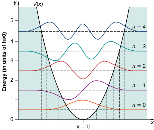
Note that ignoring the endpoints, the $0$ state has 1 hump, the $1$ state has $2$ humps, the $2$ state has $3$ humps. Recall the harmonics of a vibrating string.
Also check out osc_coherent_picker.py where you can drag a point around the plane and see the corresponding coherent state. And osc_coherent_basis.py is just like oscillator.py except it shows you the amplitudes for each coherent state in the plane, given the current state, as well as the roots of the corresponding polynomial in purple. Use i to choose a random state, c to choose a random coherent state, h to choose a random hamiltonian, e to use the oscillator hamiltonian, n to nudge the hamiltonian just a little. Use 0,1,2,3,... to check out the energy eigenstates. We can see that under the oscillator hamiltonian, the roots of the polynomial simply rotate around rigidly as a constellation in the complex position/momentum plane.
Finally, we want to emphasize again the significance of "coherent state quantization," which we've seen in the case of the quantum harmonic oscillator and the quantum spin. It turns out that we can describe a quantum harmonic oscillator state as a constellation of classical oscillator states, precisely those which are forbidden. In other words, we can interpret the quantum system as some number of copies of the classical system, which represent the classical states the quantum system can't be in, that have 0% probability of occuring. Materially, we can use coherent states to turn the quantum state into a polynomial and find the roots. This works in the case of the oscillator, where classical states refer to Gaussian wavepackets; and in the case of the spin, where classical states refer to states where all the angular momentum is concentrated in one direction. Whereas the "metaphysics" of a superposition of position states seems strange (a particle can be simultaneously in many locations?), we can perhaps find some clarity here: we can interpret a quantum state as specifying which classical states it's not. Moreover, we can describe the Schrodinger dynamics of an isolated system in terms of interactions between the constellation of classical states the system can't be in.
One is reminded of the "negative theology" of late Antiquity and the Middle Ages. For example, Maimonides urges us only to define God in negative terms, never attributing some positive quality to God, since after all, all our ideas of qualities are relative human ideas gained through comparison, which can't apply absolutely to God. So it's best to say, instead, what God isn't. We can't actually get a positive idea of God; we can only try and fail to capture God's image, realize how we failed, and thus ever so slowly characterize God by how God can't be pinned down.
Divinity aside, it is interesting that one can characterize quantum mechanics as an extension of classical mechanics that allows for systems to be defined negatively.
We can also gain a new perspective on entanglement.
Suppose we have two polynomials $f(w) = (w-1)(w-2)$ and $g(z) = (z-3)(z-4)$. We can form the tensor product through simple multiplication: $(f \otimes g)(w, z) = (w-1)(w-2)(z-3)(z-4)$.
We could form a plot of the roots of $(f \otimes g)(w, z)$:
%matplotlib inline

import numpy as np
import matplotlib.pyplot as plt
from sympy import *

z, w = symbols("z w")
p = (w-1)*(w-2)*(z-3)*(z-4)

def state_poly(q):
    global z, w
    v = q.full().T[0]
    n = int(np.sqrt(q.shape[0]))
    terms = []
    for i in range(n):
        for j in range(n):
            terms.append(v[i*n + j]*(w**i)*(z**j))
    return sum(terms)

def make_lines(roots):
    global z, w
    n_grid, L = 30, 20
    for root in roots:
        X, Y = None, None
        if w in root:
            r = root[w]
            if r.is_number:
                X = np.array([N(r)]*n_grid)
                Y = np.linspace(-L, L, n_grid)
            else:
                Y = np.linspace(-L, L, n_grid)
                X = [r.subs(z, y) for y in Y]
        if z in root:
            r = root[z]
            if r.is_number:
                X = np.linspace(-L, L, n_grid)
                Y = np.array([N(r)]*n_grid)
            else:
                X = np.linspace(-L, L, n_grid)
                Y = [r.subs(w, x) for x in X]
        plt.plot(X, Y)
    plt.show()

make_lines(solve(p))
The x-axis is the $w$ axis and the y-axis is the $z$ axis. We see two vertical lines at $1$ and $2$ cooresponding to $(w-1)(w-2)$. We get a line because $w$ must be 1 or 2 independently of $z$: the lines represents the fact that for all values of $z$, $w=1$ and $w=2$ are roots. Similarly, we have two horizontal lines at $3$ and $4$ corresponding to $(z-3)(z-4)$. We've chosen to stick with real roots since we can visualize things nicely with lines. Otherwise, we'd have to imagine: for every point in the complex plane, a map to another point on the complex plane.
What happens, though, if we add a term mixing $w$ and $z$?
%matplotlib inline
p2 = (w-1)*(w-2)*(z-3)*(z-4)*(z-w)
make_lines(solve(p2))
%matplotlib inline
p2 = (w-1)*(w-2)*(z-3)*(z-4)*(z*w-10)
make_lines(solve(p2))
In this last image, we have a relationship: $w = \frac{10}{z}$. This function has two branches, asymptoting to the $x$ and $y$ axes. Note there's a distortion in the middle as matplotlib connects the two branches.
%matplotlib inline

p3 = (w-1)*(z-1)*(z*z*w-10)
make_lines(solve(p3))
In other words, when systems are entangled we can't imagine simply: a constellation of excluded classical states of $A$ and a separate constellation of excluded classical states of $B$. Instead, we might have a joint, mutually dependent relationship: for each possible choice of excluded classical state of $A$, we can get an excluded classical state of $B$, and vice versa. In other words, the excluded classical states of $B$ are only defined up to a choice of excluded classical states of $A$. These joint root of $A$ and $B$ exclude a whole swath of the space of their togetherness.
Okay, so we have a 1D quantum harmonic oscillator. Intriguingly, we can view it as a coexistence or constellation of banned classical oscillator states; for our purposes now, however, we will view it primarily as a little guy that "counts" quanta: we can add quanta to it, subtract quanta from it, measure the number of quanta. The more quanta, the higher the energy. A general state of the oscillator is a superposition of different numbers of quanta. What is a quantum? Here, it's like a nugget of energy. It doesn't have an identity of its own: it's like the idea of a pebble: simple, indistinguishable.
Now here's a very important connection.
One of the simplest ways of understanding quantum field theory, at least at first, is via something called second quantization.
If you start with a quantum system living in some Hilbert space of dimension $d$, then you can construct a theory of a variable number of indistinguishable "copies" of that quantum system by introducing a quantum harmonic oscillator for each basis state of the original quantum system. Hence, "second quantization". (Later we'll get into the eventual difficulties with this view as regards QFT as a whole.) Note: now we're talking about not a constellation of classical systems, but a constellation of quantum systems, as it were.
As I say, in second quantized quantum mechanics, an oscillator is associated with each basis state of the original quantum system, and each oscillator counts the number of "particles" in the state it is associated with. And because we use quantum harmonic oscillators to count them, the particles so described will always be as indistinguishable as the quanta in a harmonic oscillator.
For a "bosonic field," there can be any number of particles in the same state, and the particles are always in the permutation symmetric state. For a "fermionic field," there can be at most one particle in a given state, and the particles are always in the permutation antisymmetric state. In what follows, we'll mainly be considering the bosonic case.
The point is that, remarkably, our current theories of physics regard all so-called "particles" as quanta of some quantum field, as indistinguishable, countable nuggets.
In "field theory" proper, one can think about a "quantum field" as the "first quantization" of a classical field; or as the "second quantization" of the ordinary Hilbert space of a single particle. The latter has an amplitude for each position (or momentum), and so we'll have an associated quantum harmonic oscillator at each location, counting the number of particles at that location (or in that momentum mode), and indeed: this is like a quantized model of a field, with little oscillators at each point. One can add other things to the first quantized state besides "position," like spin, and even make it relativistic. (The difficulty comes in dealing with interactions.)
But actually, the simplest "quantum field theory" involves second quantizing a little spin-$\frac{1}{2}$ particle. Such a system has two states, and so we introduce two quantum harmonic oscillators. We could say: the first oscillator keeps track of the number of $\uparrow$ quanta, and the second oscillator keeps track of the number of $\downarrow$ quanta. By construction, we'll get a theory of a variable number of permutation symmetric spin-$\frac{1}{2}$ particles. But we know what a permutation symmetric state of spin-$\frac{1}{2}$'s is! It's a spin-$j$ particle! And so, we can look at our double oscillator construction as a model of spin with variable $j$, where the $j$ value can change, and indeed, where we can have a superposition of different $j$ values.
We could write this out in "Fock" notation, but let's use polynomials first. Given two oscillators states (coeffcients suppressed):
$f(z) = z^{0} + z^{1} + z^{2} + z^{3} + \dots$
$g(w) = w^{0} + w^{1} + w^{2} + w^{3} + \dots $
We can tensor them:
$F(z, w) = z^{0}w^{0} + z^{0}w^{1} + z^{0}w^{2} + z^{0}w^{3} + \dots + z^{1}w^{0} + z^{1}w^{1} + z^{1}w^{2} + z^{1}w^{3} + \dots + z^{2}w^{0} + z^{2}w^{1} + z^{2}w^{2} + z^{2}w^{3} + \dots + z^{3}w^{0} + z^{3}w^{1} + z^{3}w^{2} + z^{3}w^{3} + \dots$
But this can be rearranged:
$F(z, w) = \Big{\{} z^{0}w^{0} \Big{\}} + \Big{\{} z^{1}w^{0} + z^{0}w^{1} \Big{\}} + \Big{\{} z^{2}w^{0} + z^{1}w^{1} + z^{0}w^{2} \Big{\}} + \Big{\{} z^{3}w^{0} + z^{2}w^{1} + z^{1}w^{2} + z^{0}w^{3} \Big{\}} + \dots$
In other words, we can regard the two variable polynomial as a sum of homogenous polynomials, of degree $0, 1, 2, 3, 4, \ldots$. (Recall our use of homogenous polynomials way back during our discussion of the Majorana representation.) Each such sector of the Hilbert space, corresponding to a given total $n$, can be interpreted as a spin-$\frac{n}{2}$ state. In other words, $n$ is just $2j$, the number of stars.
The correspondence between the occupation number basis of the two oscillators, the spin basis states in the $\mid j, m \rangle$ representation, and the states of $2j$ symmeterized spin-$\frac{1}{2}$'s is:
Total Number: 0
$\begin{matrix}\mid 0 0 \rangle & \mid 0, 0 \rangle & \mid 0 \rangle \end{matrix}$
Total Number: 1
$\begin{matrix} \mid 1 0 \rangle & \mid \frac{1}{2}, \frac{1}{2} \rangle & \mid \uparrow \rangle \\ \mid 0 1 \rangle & \mid \frac{1}{2}, -\frac{1}{2} \rangle & \mid \downarrow \rangle \end{matrix}$
Total Number: 2
$\begin{matrix} \mid 2 0 \rangle & \mid 1, 1 \rangle & \mid \uparrow \uparrow \rangle \\ \mid 1 1 \rangle & \mid 1, 0 \rangle & \mid \uparrow \downarrow \rangle + \mid \downarrow \uparrow \rangle \\ \mid 0 2 \rangle & \mid 1, -1 \rangle & \mid \downarrow \downarrow \rangle \end{matrix}$
Total Number: 3
$\begin{matrix} \mid 3 0 \rangle & \mid \frac{3}{2}, \frac{3}{2} \rangle & \mid \uparrow \uparrow \uparrow \rangle \\ \mid 2 1 \rangle & \mid \frac{3}{2}, \frac{1}{2} \rangle & \mid \uparrow \uparrow \downarrow \rangle + \mid \uparrow \downarrow \uparrow \rangle + \mid \downarrow \uparrow \uparrow \rangle \\ \mid 1 2 \rangle & \mid \frac{3}{2}, -\frac{1}{2} \rangle & \mid \downarrow \downarrow \uparrow \rangle + \mid \downarrow \uparrow \downarrow \rangle + \mid \uparrow \downarrow \downarrow \rangle \\ \mid 0 3 \rangle & \mid \frac{3}{2}, -\frac{3}{2} \rangle & \mid \downarrow \downarrow \downarrow \rangle \end{matrix}$
And so on...
We can upgrade any $2$ x $2$ operator on the spin-$\frac{1}{2}$ Hilbert space to act globally on the Hilbert space of the oscillators via simple map:
$ \textbf{O} = \sum_{i, j} a_{i}^{\dagger} O_{i, j} a_{j} $
Or: $\textbf{O} = \begin{pmatrix} a_{0}^{\dagger} & a_{1}^{\dagger} \end{pmatrix} \begin{pmatrix} a & b \\ c & d \end{pmatrix} \begin{pmatrix} a_{0} \\ a_{1}\end{pmatrix}$, where I emphasize that the $a_{i}$'s and $a_{i}^{\dagger}$'s are themselves operators.
So that:
$X = \begin{pmatrix} a_{0}^{\dagger} & a_{1}^{\dagger} \end{pmatrix} \begin{pmatrix} 0 & 1 \\ 1 & 0 \end{pmatrix} \begin{pmatrix} a_{0} \\ a_{1}\end{pmatrix} = \begin{pmatrix} a_{0}^{\dagger} & a_{1}^{\dagger} \end{pmatrix} \begin{pmatrix} a_{1} \\ a_{0}\end{pmatrix} = a_{0}^{\dagger}a_{1} + a_{1}^{\dagger}a_{0}$
$Y = \begin{pmatrix} a_{0}^{\dagger} & a_{1}^{\dagger} \end{pmatrix} \begin{pmatrix} 0 & -i \\ i & 0 \end{pmatrix} \begin{pmatrix} a_{0} \\ a_{1}\end{pmatrix} = \begin{pmatrix} a_{0}^{\dagger} & a_{1}^{\dagger} \end{pmatrix} \begin{pmatrix} -ia_{1} \\ ia_{0}\end{pmatrix} = -ia_{0}^{\dagger}a_{1} + ia_{1}^{\dagger}a_{0}$
$Z = \begin{pmatrix} a_{0}^{\dagger} & a_{1}^{\dagger} \end{pmatrix} \begin{pmatrix} 1 & 0 \\ 0 & -1 \end{pmatrix} \begin{pmatrix} a_{0} \\ a_{1}\end{pmatrix} = \begin{pmatrix} a_{0}^{\dagger} & a_{1}^{\dagger} \end{pmatrix} \begin{pmatrix} a_{0} \\ -a_{1}\end{pmatrix} = a_{0}^{\dagger}a_{0} - a_{1}^{\dagger}a_{1}$
If we upgrade the $X$ operator, for example, it will act as an $X$ operator on each of the spin-$j$ subspaces. If we use it to rotate, it'll rotate all the subspaces at the same time.
We can also form a creation operator that creates a star at a given location. Given some spinor $\begin{pmatrix} \alpha \\ \beta \end{pmatrix}$, the star creation operator is $a_{star}^{\dagger} = \alpha a_{0}^{\dagger} + \beta a_{1}^{\dagger}$.
We could decompose a spin-$j$ state into $2j$ spinors, and then lift the constellation into the double harmonic ocillator Hilbert space one star at a time. Or we could form a homogenous polynomial in the creation operators:
$a_{constellation}^{\dagger} = \sum_{m=-j}^{j} \begin{pmatrix}2j \\ j+m \end{pmatrix} c_{j+m} (a_{0}^{\dagger})^{j-m}(a_{1}^{\dagger})^{j+m}$
where the $c_{i}$'s are the components of the $\mid j, m \rangle$ state: $\begin{pmatrix} c_{0} \\ c_{1} \\ c_{2} \\ \vdots \end{pmatrix}$. Recall the binomial coefficient enters into the game due to the relationship between the roots and coefficients of a polynomial. Majorana returns! In fact, Schwinger learned about Majorana's representation at some point in the 30's and 40's, and it bugged him so much he invented a lot of this.
import qutip as qt
import numpy as np
import vpython as vp
scene = vp.canvas(background=vp.color.white)

def spinor_xyz(s):
    return np.array([qt.expect(qt.sigmax(), s),\
                     qt.expect(qt.sigmay(), s),\
                     qt.expect(qt.sigmaz(), s)])

a = (qt.basis(2,0)-1j*qt.basis(2,1)).unit()
xyz = spinor_xyz(a)
vsphere = vp.sphere(pos=vp.vector(2,0,0), color=vp.color.blue, opacity=0.3)
varrow = vp.arrow(pos=vsphere.pos, axis=vp.vector(*xyz))

x, y = a.full().T[0].real
vpt = vp.sphere(pos=vp.vector(x,y,0), radius=0.1, color=vp.color.yellow, make_trail=True)

dt = 0.001
while True:
    a = np.exp(1j*dt)*a
    x, y = a.full().T[0].real
    vpt.pos = vp.vector(x,y,0)
    vp.rate(1000)
A word to the wise: a photon is technically a spin-$1$ particle, but because it's massless, it has only two possible states.
Finally, we have a new way of thinking about the duality between the plane and the sphere: the same state can represent the polarization of a massless particle (plane) or the spin of a massive particle (spin).
One nice consequence of this duality is that we can build quantum computers out of spins and also quantum computers out of light, and easily translate between them. I can represent my spin operators on the photons; and the photonic operators on the spins. And so, the one can simulate the other. Of course, this is more profound than a mere classical simulation. If I load a given quantum state into a quantum computer made of spins, of light, of whatever, this won't in principle affect its entanglement to other systems. So when you download something from the quantum internet onto a quantum computer even with a different architecture, it really is that unique non-clonable quantum state, and not merely a representation, a copy of it, as would be the case if you loaded some classical data into your computer.
One thing that is also clear is that there can be many perspectives conceptually on the same quantum system. We have a constellation on the sphere. Is it a spin-$j$ particle? Is it $2j$ spin-$\frac{1}{2}$'s, is it two quantum harmonic oscillators? Or is it the orbital angular momentum of a light beam? The interpretation is physically fixed by how the system interacts with the rest of the world; and conceptually each new interpretation brings with it a whole unheralded set of ideas and connections to the rest of the world.
Check out spin_oscillators.py! One can choose a max number of quanta in each of the two oscillators, as well as a random spin state to be loaded into the double oscillator Hilbert space, and a Hamiltonian to evolve with. One sees above a red sphere representing the original spin state (just to make sure it's loaded in correctly!), and below a series of blue spheres representing the spin-$0$, spin-$\frac{1}{2}$, spin-$1$, $\dots$ states that the Hilbert space decomposes into. Their opacity is just the norm of that sector. In the middle, one sees the plane, with little arrows at each point representing the amplitude at that location. Using the keyboard, one can measure the X, Y, Z, N (number), and Q (position) operators with "x", "y", "z", "n", and "q". "i" gives you a random state, "h" picks a random hamiltonian, "e" returns you to the oscillator hamiltonian, "s" picks X, Y, Z to be hamiltonian. Play around with it! (Note because we're using truncated oscillators, the decompositions into spins is symmeterical.)
Spin is all about representations of the group SU(2), which is the double cover of 3D rotations. We can view the spin-$\frac{1}{2}$ representation as a kind of template, and build up the higher spin representations as "constellations" of spin-$\frac{1}{2}$'s. This is done systematically through second quantizing the basic representation.
Instead of using SU(2), we could use SU(3), which acts on 3D complex states, and then we'd have 3 harmonic oscillators, but actually we'd need 6, since SU(3) is rank 2. Indeed, the same pattern can be applied to SU(N). Generally speaking, we can construct theories of a variable number of indistinguishable "particles" with different symmeteries. The oscillator space can be interpreted as a superposition of higher order representations, each of which can be itself represented as an unordered collection of "stars," or basic states, to be symmeterized. Thus the atomic pattern continues.
Furthermore, in a second quantized context, we could regard any measurement as, in fact, the measurement of the number of particles in a certain state. We could rephrase a spin measurement along the $Z$ axis in terms of the of "the number of quanta in the $\uparrow$ oscillator" and "the number of quanta in the $\downarrow$ oscillator" (at a certain location). Indeed, we could rotate the creation and annihilation operators themselves to count $\rightarrow$ and $\leftarrow$ quanta instead.
Due to second quantization, we can think about any measurement, in some sense, as being reducible to the measurement of some number operator.
In a way, we've come full circle. We can now contextualize our pebbles as counting the number of indistinguishable quanta of some mode of a quantum field. And any actual distinguishable clay pebble has emerged in the limit of this quantum theory.
Check out qft.py for an very rudimentary example of a 1D quantum field theory. Choose the number of discrete positions, the max num of excitations per oscillator. Each position also carries a spin. In fact, since we have to introduce two oscillators per position, we can have a variable spin-$j$ at each location.
The height of the cylinders is the expectation value of the number of particles at each location. Below, you see the expected spin axis at that location, as well as the expected values of the number operators for up and down quanta.
We begin by upgrading an oscillator coherent state with a definite spin, and also upgrading the oscillator hamiltonian to an operator that acts on the field. Also try simply creating a "star" at a given location out of the vacuum. The free field hamiltonian is given by the sum of the momentum oscillator hamiltonians.
Crucially, by building operators out of the creation and annihilation operators at a given position, one can guarantee that spacelike separated operators commute: this is useful if for whatever reason there fail to be tensor products in the Hilbert space.
Obviously, we could add other dimensions of space and other internal symmetries. We could try to make the theory relativistic. In the general case, once you include interactions, there is a theorem (Haag's theorem), which says that the resulting theory will be unitarily inequivalent to one built out of oscillators. We'll return to these ideas in the next section.