We begin with an interesting observation.
Consider some n x n unitary matrix, and look at its first two columns. They will be orthogonal complex vectors.
import qutip as qt
import numpy as np

n = 4
U = qt.rand_unitary(n)
col0, col1 = U[:,0], U[:, 1]
print(np.vdot(col0, col1))
Then form n spinors, by taking the first component of each from the first column, and the second component of each from the second column.
$ \begin{pmatrix} a & b & c & d \\ e & f & g & h \\ i & j & k & l \\ m & n & o & p \end{pmatrix} \rightarrow \begin{pmatrix} a & b \\ e & f \\ i & j \\ m & n \end{pmatrix} \rightarrow \Big{\{} \begin{pmatrix} a \\ b \end{pmatrix}, \begin{pmatrix} e \\ f \end{pmatrix}, \begin{pmatrix} i \\ j \end{pmatrix}, \begin{pmatrix} m \\ n \end{pmatrix} \Big{\}}$
These spinors in general won't be normalized.
spinors = [qt.Qobj(np.array([col0[i], col1[i]])) for i in range(n)]
print([s.norm() for s in spinors])
Here's the interesting observation. If you convert all those spinors into $(x, y, z)$ vectors, and add them up: their sum will always be 0.
def spinor_xyz(spinor):
    return np.array([qt.expect(qt.sigmax(), spinor), qt.expect(qt.sigmay(), spinor), qt.expect(qt.sigmaz(), spinor)])

xyzs = [spinor_xyz(s) for s in spinors]
print(sum(xyzs))
There is a famous theorem due to Minkowski about polyhedra. He tells us that you can describe a polyhedron in terms of its vertices, sure, but you can also uniquely specify a polyhedron by giving: the unit normals to its faces, $\vec{u_{i}}$, and the areas of those faces $a_{i}$.
Given $n$ faces, you can package up this information into $n$ vectors: $a_{i}\vec{u_{i}}$: each such vector points in the direction normal to a face, and has a length equal to the area of the face. The condition that the polyhedron is legit, in other words, that it's closed is just:
$\sum_{i} a_{i}\vec{u_{i}} = 0$
We can therefore see that we can interpret the first two columns of our unitary matrix as specifying a polyhedron: the corresponding spinors the unit normals scaled by the areas. In fact, any two orthogonal complex vectors specify a polyhedron in terms of the components paired off, interpreted as spinors.
import qutip as qt
import numpy as np
import examples.polyhedrec as polyhedrec
from examples.vhelper import *
scene = vp.canvas(background=vp.color.white)

n = 6
U = qt.rand_unitary(n)

def unitary_spinors(U):
    col0, col1 = U[:,0], U[:, 1]
    return [qt.Qobj(np.array([col0[i], col1[i]])) for i in range(n)]

def spinor_xyz(spinor):
    return np.array([qt.expect(qt.sigmax(), spinor), qt.expect(qt.sigmay(), spinor), qt.expect(qt.sigmaz(), spinor)])

def make_poly(spinors):
    xyzs = [spinor_xyz(s) for s in spinors]
    areas = [np.linalg.norm(xyz) for xyz in xyzs]
    unormals = [xyz/areas[i] for i, xyz in enumerate(xyzs)]
    return polyhedrec.reconstruct(unormals, areas)

vp.sphere(radius=0)
VisualPolyhedron(make_poly(unitary_spinors(U)))
In the above, we use the "polyhedrec" library (available here) to reconstruct the polyhedron from its areas and unit normals: the calculation is a little involved! Also, note that the polyhedron is defined up to 3D rotations. (Also, for $n = 3$, we get a polygon in the plane, which will give the library some trouble, etc.)
Now one thing that this implies is that there is an action of $U(N)$ on polyhedra (where $N$ is the number of faces).
import qutip as qt
import numpy as np
import examples.polyhedrec as polyhedrec
from examples.vhelper import *
scene = vp.canvas(background=vp.color.white)

n = 6
dt = 0.001
U = qt.rand_unitary(n)
V = (-1j*qt.rand_herm(n)*dt).expm()

def unitary_spinors(U):
    col0, col1 = U[:,0], U[:, 1]
    return [qt.Qobj(np.array([col0[i], col1[i]])) for i in range(n)]

def spinor_xyz(spinor):
    return np.array([qt.expect(qt.sigmax(), spinor), qt.expect(qt.sigmay(), spinor), qt.expect(qt.sigmaz(), spinor)])

def make_poly(spinors):
    xyzs = [spinor_xyz(s) for s in spinors]
    areas = [np.linalg.norm(xyz) for xyz in xyzs]
    unormals = [xyz/areas[i] for i, xyz in enumerate(xyzs)]
    return polyhedrec.reconstruct(unormals, areas)

vpoly = VisualPolyhedron(make_poly(unitary_spinors(U)))

print("total area: %f" % sum([np.linalg.norm(spinor_xyz(s)) for s in unitary_spinors(U)]))
for t in range(100):
    U = V*U
    vpoly.update(make_poly(unitary_spinors(U)))
    vp.rate(500)
print("total area: %f" % sum([np.linalg.norm(spinor_xyz(s)) for s in unitary_spinors(U)]))
In fact, we can see that not only does the action of a unitary on the polyhedron preserve the closure constraint, but also: it preserves the total surface area of the polyhedron!
Now suppose we had any old random set of vectors in 3D, which doesn't necessarily satisfy the closure constraint. It turns out we can easily calculate a Lorentz boost, which acts on the spinors, and closes the polyhedron.
We form the projector for each spinor, and sum them all: $S = \sum_{i} \mid \phi_{i} \rangle \langle \phi_{i} \mid$. We then use singular value decomposition to split $S$ into $S = UDV$, where $U$ and $V$ are unitaries, and $D$ is a diagonal matrix. We then form a boost $B = det(D)^{-\frac{1}{4}}U\sqrt{D}$, and actually the boost we want is just the inverse: $B^{-1}$. If we apply this $SL(2, \mathbb{C}$ matrix to each spinor, we'll end up with a closed polyhedron.
One implication is that if we imagine our spinors refering to the directions and energies of incoming photons on the celestial sphere, there's always a velocity we could be traveling so that the sum of the energy/direction vectors is 0: and they form a closed polyhedron.
import qutip as qt
import numpy as np

def spinor_xyz(spinor):
    return np.array([qt.expect(qt.sigmax(), spinor), qt.expect(qt.sigmay(), spinor), qt.expect(qt.sigmaz(), spinor)])

def close_spinors(spinors):
    S = sum([spinor*spinor.dag() for spinor in spinors])
    U, d, V = np.linalg.svd(S.full())
    D = np.diag(d)
    rho = np.linalg.det(D)
    B = np.dot(U, np.sqrt(D)*rho**(-1./4.))
    Bi = qt.Qobj(np.linalg.inv(B))
    return Bi, [Bi*spinor for spinor in spinors]

def check_closure(spinors):
    return sum([spinor_xyz(s) for s in spinors])

n = 5
spinors = [np.random.randn(1)[0]*qt.rand_ket(2) for i in range(n)]
print("closure: %s" % check_closure(spinors))
boost, closed_spinors = close_spinors(spinors)
print("closure: %s" % check_closure(closed_spinors))
Furthermore, it's worth noting we can act with our unitary directly on the set of spinors. For each spinor $\phi_{i}$:
$\phi_{i} \rightarrow \sum_{i,j} U_{i,j}\phi_{j}$
import qutip as qt
import numpy as np
import examples.polyhedrec as polyhedrec
from examples.vhelper import *
scene = vp.canvas(background=vp.color.white)

n = 6
dt = 0.001
U = qt.rand_unitary(n)
V = (-1j*qt.rand_herm(n)*dt).expm()

def unitary_spinors(U):
    col0, col1 = U[:,0], U[:, 1]
    return [qt.Qobj(np.array([col0[i], col1[i]])) for i in range(n)]

def spinor_xyz(spinor):
    return np.array([qt.expect(qt.sigmax(), spinor), qt.expect(qt.sigmay(), spinor), qt.expect(qt.sigmaz(), spinor)])

def make_poly(spinors):
    xyzs = [spinor_xyz(s) for s in spinors]
    areas = [np.linalg.norm(xyz) for xyz in xyzs]
    unormals = [xyz/areas[i] for i, xyz in enumerate(xyzs)]
    return polyhedrec.reconstruct(unormals, areas)

spinors = unitary_spinors(U)
vpoly1 = VisualPolyhedron(make_poly(spinors), [-1, 0, 0])
vpoly2 = VisualPolyhedron(make_poly(spinors), [1, 0, 0])

for t in range(50):
    U = V*U
    spinors = [sum([V.full()[i][j]*spinors[j]\
                for j in range(n)])\
                   for i in range(n)]
    vpoly1.update(make_poly(unitary_spinors(U)))
    vpoly2.update(make_poly(spinors))
    vp.rate(500)

s0, s1 = spinors, unitary_spinors(U)
print(np.array([np.isclose((s0[i]-s1[i]).full().T[0], np.array([0,0])).all() for i in range(n)]).all())
So it's interesting that we can fully specify a classical polyhedron in terms of its unit normals and areas, expressed for example as a set of spinors. This provides a clue for how to quantize polyhedra and obtain the quantum polyhedron, which we can regard as an "atom of space". In fact, we've already done it, we just didn't realize what we were doing!
The basic idea is this. We quantize each spinor, representing a polyhedral face, as a spin-$j$ particle. The $J^{2}$ operator $J^{2} = X^{2} + Y^{2} + Z^{2}$ becomes the area operator (squared) of the face. We then consider the tensor product of the $n$ spin-$j$ particles representing the $n$ faces. We form the total spin operator $J_{total}^{2} = (\sum_{i} X_{i})^{2} + (\sum_{i} Y_{i})^{2} + (\sum_{i} Z_{i})^{2}$, and demand that our states live in the angular momentum $0$ eigenspace. This constraint is the quantum equivalent of the closure constraint, as we will see.
We've actually already considered this.
For example, suppose we have four spin-$\frac{1}{2}$ states. The angular momentum 0 subspace of their tensor product is two dimensional.
$H_{\frac{1}{2}} \otimes H_{\frac{1}{2}} \otimes H_{\frac{1}{2}} \otimes H_{\frac{1}{2}} = (H_{0} \oplus H_{0}) \oplus (H_{1} \oplus H_{1} \oplus H_{1}) \oplus (H_{2})$.
This means that we can use a single qubit to parameterize the angular momentum 0 subspace of four spin-$\frac{1}{2}$ states. Each of the qubit basis vectors is sent to one of the two eigenvectors of $J_{total}^{2}$ with eigenvalue 0. In general, this subspace will be larger (or smaller), but we could always use a nominal spin-$j$ particle to parameterize the angular momentum 0 subspace of the tensor product. Depending on the $j$ values of the tensored spins, there may not even be an angular momentum 0 subspace at all: and so these spins can't form the faces of a quantum polyhedron.
For each face spin, we have a set of $X$, $Y$, $Z$ operators, each tensored appropriately with identities so they act on only their own spin. Now you might think that the vector corresponding to each face would just be given by the expectation values of X, Y, Z on the face spin, but that's not how it works.
Instead: define the following "inner product operators" between two spins $\Phi_{i}$ and $\Phi_{j}$:
$ \Phi_{i} \cdot \Phi_{j} = X_{i}X_{j} + Y_{i}Y_{j} + Z_{i}Z_{j}$
For concreteness, suppose we have four faces. Consider the following matrix of operators:
$\begin{pmatrix} \Phi_{0} \cdot \Phi_{0} & \Phi_{0} \cdot \Phi_{1} & \Phi_{0} \cdot \Phi_{2} & \Phi_{0} \cdot \Phi_{3} \\ \Phi_{1} \cdot \Phi_{0} & \Phi_{1} \cdot \Phi_{1} & \Phi_{1} \cdot \Phi_{2} & \Phi_{1} \cdot \Phi_{3} \\ \Phi_{2} \cdot \Phi_{0} & \Phi_{2} \cdot \Phi_{1} & \Phi_{2} \cdot \Phi_{2} & \Phi_{2} \cdot \Phi_{3} \\ \Phi_{3} \cdot \Phi_{0} & \Phi_{3} \cdot \Phi_{1} & \Phi_{3} \cdot \Phi_{2} & \Phi_{3} \cdot \Phi_{3} \end{pmatrix}$
Along the diagonal, we have the area operators. And the off-diagonal terms correspond to all the possible inner products between the face vectors, which relate to the cosines of the angles between the faces: we can think of these like "angle" operators.
Given some polyhedron state $\mid \pi \rangle$, we can take its expectation values on each of the operators above, and form a matrix out of them:
$G_{i,j} = \langle \pi \mid \Phi_{i} \cdot \Phi_{j} \mid \pi \rangle$
We then decompose $G$ using the singular value decomposition: $G = UDV$. We consider the first three rows of $V$, and turn them into columns and make a matrix $V^{\prime}$. We also consider the first three columns/rows of $\sqrt{D}$, and form $D^{\prime}$. We then form the matrix:
$ M = V^{\prime}D^{\prime}$.
The rows of this matrix will be the (x, y, z) coordinates of the face vectors. In other words, their norms will be the areas of the faces, and their directions will be the unit normals to each face.
The quantum closure constraint guarantees that these (x, y, z) vectors all sum to 0, and so represent a closed polyhedron: although recall that now these vectors are obtained via the expectation values of quantum operators!
Before we demonstrate the quantum version, let's just make sure that this procedure works in the case of a classical polyhedron!
import qutip as qt
import numpy as np
import examples.polyhedrec as polyhedrec

def unitary_spinors(U):
    col0, col1 = U[:,0], U[:, 1]
    return [qt.Qobj(np.array([col0[i], col1[i]])) for i in range(n)]

def spinor_xyz(spinor):
    return np.array([qt.expect(qt.sigmax(), spinor), qt.expect(qt.sigmay(), spinor), qt.expect(qt.sigmaz(), spinor)])

def vectors(spinors):
    return [spinor_xyz(s) for s in spinors]

def inner_products(vectors):
    return np.array([[np.dot(vectors[i], vectors[j]) for j in range(len(vectors))] for i in range(len(vectors))])

def recover_vectors(G):
    U, D, V = np.linalg.svd(G)
    M = np.dot(V[:3].T, np.sqrt(np.diag(D[:3])))
    return [m for m in M]

n = 6
U = qt.rand_unitary(n)

vecs = vectors(unitary_spinors(U))
G = inner_products(vecs)
vecs2 = recover_vectors(G)
G2 = inner_products(vecs2)

print(G)
print()
print(G2)
We can see that if we have a bunch of vectors satisfying the closure constraint, we can form $G$, the matrix of the inner products between them. We can then recover the vectors via the above method up to a 3D rotation. Indeed, we don't get exactly the vectors back, but we can see that they are the same up to a 3D rotation, since the $G$ matrix formed from the recovered vectors is identical.
Putting it all together, we can construct a quantum polyhedron in the following way. We pick $j$ values for each of the $n$ faces, and form the tensor product of $n$ spins, one for each face. We constrain ourselves to work only in the spin-$0$ subspace of the tensor product, and so depending on the dimensionality $d$ we can represent this as a "qudit" of $d$ dimensions. We construct the inner product operators out of all the $X_{i}$'s, $Y_{i}$'s, and $Z_{i}$'s, and given some polyhedron state $\mid \pi \rangle$, we form the matrix of the expectation values on all these operators. We then recover the face vectors using the singular value decomposition. At last, using Minkowski's Theorem, we can construct a polyhedron out of these statistical averages. Because we're stuck in the spin-$0$ subspace, the face vectors will always form a (possibly degenerate) closed polyhedron.
In fact, for efficiency's sake, we can downgrade all the inner product operators to act on the qudit that spans the spin-$0$ subspace instead of the much larger tensor product. We'll already have to construct an operator $S$ that takes the qudit state to a state in the original tensor product, so that $\mid \pi \rangle = S\mid q \rangle$. We can use this same operator to upgrade operators that act on $\mid q \rangle$ to operators that act on $\mid \pi \rangle$: $O_{big} = SO_{tiny}S^{\dagger}$, and downgrade operators that act on $\mid \pi \rangle$ to operators that act on $\mid q \rangle$: $O_{tiny} = S^{\dagger}O_{big}S$. And so, we can downgrade all our inner product operators to act on the qudit.
And actually, this is a good idea anyway, since the eigenstates of inner product operators acting on the tensor product don't all live in the spin-$0$ subspace. So downgrading the operators makes sure their eigenstates all live in the spin-$0$ subspace. Lest this worry you, this doesn't effect the expectation values in any way, and if you downgrade one of these operators and upgrade it back, the resulting operator commutes with the original operator.
We can then evolve our quantum polyhedron under some unitary matrix just as we could evolve our classical polyhedron, by choosing some unitary that acts on the underlying qudit.
Check out quantum_polyhedron.py!
Choose a set of $j$ values for your faces. You can then evolve the polyhedron in time using a Hamiltonian that acts on the underlying qudit: p.evolve(H=qt.rand_herm(p.d), dt=0.01, t=1000). You can also measure one of the operators, for example: p.measure(p.INNER_PRODUCTS[0][1], tiny=False). Operators are assumed to act on the tensor product, and are automatically downgraded to act on the qudit. If you already have a "tiny" operator, set tiny=True. If the polyhedron is degenerate, or if something otherwise goes wrong, the underlying vectors will be displayed instead of the polyhedron. Finally, you'll notice that the polyhedron glitches out from time to time: this is because the polyhedron is only defined up to 3D rotation, and so when we recover the polyhedron at each time step, we might end up with a arbitrarily rotated version. It would be nice to easily calculate the 3D rotation that will make sure to align the orientation of the polyhedron over time, but it's a little tricky!
Note as well that just as before: the total area of the polyhedron is preserved under unitary evolution, and under measurements too, for that matter. And actually, it's a little more than before: the areas of each of the individual faces is preserved as well.
Although we can visualize a quantum polyhedron as a classical polyhedron built of expectation values, don't be mislead: there is something distinctively quantum going on here.
The crucial fact is that, in general, the inner product operators don't commute. This means that we can't "simultaneously know" all the angles between the faces of the quantum polyhedron at the same time.
For example, if we measure the angle between the first two faces, we'll end up in an eigenstate of that operator. But this will lead to uncertainty in the angles between the other faces: we won't be in an eigenstate of those operators.
from examples.quantum_polyhedron import *

p = QuantumPolyhedron([1/2, 1/2, 1/2, 1/2])
IP01 = p.INNER_PRODUCTS_[0][1]
IP12 = p.INNER_PRODUCTS_[1][2]
print("Eigenvalues for angle between faces 0 and 1: %s" % IP01.eigenstates()[0])
print("Eigenvalues for angle between faces 1 and 2: %s" % IP12.eigenstates()[0])
print()
print(p.inner_products())
print()
p.measure(p.INNER_PRODUCTS[0][1])
print()
print(p.inner_products())
We can see above that if we measure the inner product between faces 0 and 1 or between faces 1 and 2, we can either $-\frac{3}{4}$ or $\frac{1}{2}$ as eigenvalues. If we measure the first operator, we collapse to one of its eigenstate. So the $G_{0,1}$ entry of the matrix goes to $-\frac{3}{4}$ or $\frac{1}{2}$: but we also see that if we do so, then the $G_{1,2}$ entry of the matrix will never be one of the eigenvalues! And hence, there is a quantum uncertainty about the inner product between them: in fact, in this case, the matrix entry is either $-\frac{1}{2}$ or $0$.
In fact, we see here that when the angle between 0 and 1 is definite, then so is the angle between 2 and 3. So we can know two of the angles at once, but not the others!
In other words, the polyhedron can't simulatenously be in an eigenstate of all its inner product operators, and so there is a complementarity between knowing the different angles between pairs of faces. And yet, from the expectation values of the quantum polyhedron, we can form a classical polyhedron which satisfies the closure condition.
It's analogous to the case of spin, say, a qubit. We can form a representation of its rotation axis as an (x, y, z) vector formed from the expectation values of the X, Y, Z operators. This is just the state of a classical spinning object, but it is built out of statistical averages. The really quantum part comes in when we go to measure the spin: the X, Y, Z operators don't commute, and so if we collapse to an X eigenstate, this will lead to uncertainty in Y and Z: we'll end up in a superposition of Y or Z eigenstates. So that choosing to measure along X, Y, or Z precludes us from knowing the spin in the other directions. Nevertheless, being in an X eigenstate, with uncertainty in Y and Z, corresponds to: yet another classical state of the spinning object, this time with its rotation axis pointing along the X direction. Moreover, we can recover the original state by performing the experiment many times on identically prepared states, measuring X, Y, Z in turn, over and over again.
Similarly, in the case of a quantum polyhedron, we can form a representation of it as a classical polyhedron, built out of expectation values. The inner product operators don't all commute, and so if we collapse to an eigenstate of one of them, this leads to uncertainty in the other operators, which precludes us from knowing those angles. By measuring the one angle, we've renounced knowledge of the others. Nevertheless, the resulting state corresponds to: yet another classical polyhedron in terms of the expectation values. Moreover, we can recover the original state by performing repeated experiments on identically prepared polyhedra, measuring the different angles in turn, over and over again.
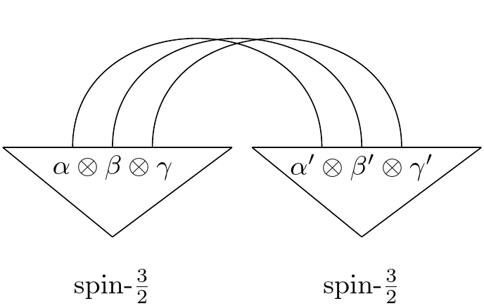
One way of interpreting a tensor product of spins in the spin-$0$ subspace is as an interaction vertex that preserves angular momentum. In other words, it represents a possible interaction such that the total angular momentum coming in is the same as the total angular momentum going out.
To see this, let us have recourse to our symmeterized spinor formalism for a moment.
Suppose we have two spin-$\frac{1}{2}$ states and we want to contract them in an angular momentum invariant way.
Back in the string diagram days, we had a way of contracting states: the cup.
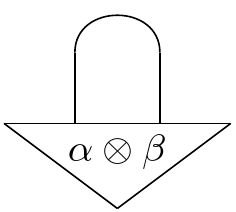
When we work with spins, it's useful to use a different set of cups and caps:
Instead of using the $\mid \uparrow \uparrow \rangle + \mid \downarrow \downarrow \rangle$ state, we use the antisymmetric state. This is often called $\epsilon$.
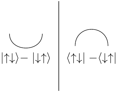
Suppose we want to contract two spin-$j$ states in an angular momentum way. What's the right cap? For concreteness, take two spin-$\frac{3}{2}$ states. Construct the permutation symmetric tensor product representation of each. Each state has three stars, and so can be represented as a symmeterized tensor product of three spin-$\frac{1}{2}$ states. Use the antisymmetric cup to contract each of the spin-$\frac{1}{2}$'s with their pair on the other side.
We can also see that we can use the $\epsilon$ to raise and lower indices: to go from bra's to ket's in an angular momentum invariant way. The point is that if you yank a spin, its spin axis should flip: incoming and outgoing spins should have opposite senses.
If we wanted to work with the spin states in the $\mid j, m \rangle$ representations directly, we could imagine constructing the $\epsilon_{j}$ by tensoring $2j$ copies of the $\epsilon_{\frac{1}{2}}$ together, permuting them so that all $\epsilon$ inputs are on the left and all the $\epsilon$ outputs are on the right. Call this $\epsilon_{sym-j}$. We have some $S$, for which $S\mid\psi_{sym}\rangle = \mid\psi_{spin}\rangle$: it acts on a permutation symmetric state of $2^{2j}$ dimensions and downgrades us to the $2j+1$ dimensional $\mid j, m\rangle$ state. So we apply $(S \otimes S)$ to $\epsilon_{sym-j}$ to get $\epsilon_{j}$, which let's us contract two spin-$j$ particles directly.
import qutip as qt
import numpy as np
from examples.magic import *
from examples.quantum_polyhedron import *

def repair(q):
    q.dims[1] = [1]*len(q.dims[0])
    return q

def epsilonj(j):
    n = int(2*j)
    epsilons = qt.tensor(*[np.sqrt(2)*qt.bell_state("11")]*(n))
    epsilons = epsilons.permute(list(range(0, 2*n, 2))+list(range(1, 2*n, 2)))
    S = sym_spin(n)
    return repair(qt.tensor(S, S)*epsilons)

def contract(qpoly, input_spin, index, verbose=True, restore_norm=True):
    input_j = qpoly.js[index]
    epsilon = (np.sqrt(2*input_j +1) if restore_norm else 1)*epsilonj(input_j)

    state = qt.tensor(epsilon, input_spin, qpoly.zero_map*qpoly.spin)
    output_spins = qt.tensor_contract(state, (1, index+3))
    output_spins = qt.tensor_contract(output_spins, (0, 1))
    if verbose:
        X0, Y0, Z0, J20 = make_total_spin([input_j])
        removed_indices = qpoly.js[:]
        del removed_indices[index]
        X1, Y1, Z1, J21 = make_total_spin(removed_indices)

        input_xyz = np.array([qt.expect(sum(X0), input_spin),\
                              qt.expect(sum(Y0), input_spin),\
                              qt.expect(sum(Z0), input_spin)])
        output_xyz = np.array([qt.expect(sum(X1), output_spins),\
                               qt.expect(sum(Y1), output_spins),\
                               qt.expect(sum(Z1), output_spins)])
        print("input ang mo: %s " % input_xyz)
        print("output ang mo: %s " % output_xyz)
        print("difference: %s" % (input_xyz-output_xyz))
    return repair(output_spins)

p = QuantumPolyhedron([1/2,1/2,1/2,1/2])
contract(p, qt.rand_ket(2), 0)
Above we have a quantum tetrahedron with four spin-$\frac{1}{2}$'s as faces. We consider an incoming spin-$\frac{1}{2}$ at random. Using the $\epsilon$, we contract the incoming spin with the first face. This steers us to a state of three outgoing spin-$\frac{1}{2}$'s, and comparing the angular momentum of the incoming spin with the total angular momentum of the outgoing spins, we find that they are exactly equal. This would not be true if the four spins corresponding to the faces weren't in the spin-$0$ subspace. In other words, the closure of our polyhedron corresponds to the conservation of angular momentum.
Let's dig a little deeper.
Below we have code that lets you contract arbitrary numbers of spins onto the faces of a polyhedron. In general, however, the norm of the resulting state may not be 1: this happens when it's impossible to satisfy the angular momentum constraint given the input up to a scalar. The more you contract it may even be impossible to satisfy the angular momentum constraint at all. You may be asking too much if you just choose any old input spins. If you contract all the spins, you get a scalar: the probability that those incoming spins would emerge as the output spins identical to the spins of the polyhedron. In other words, that those spins, coming together, would form the polyhedron: or that: those spins could pass through the polyhedron unaffected, merely flipping from incoming to outgoing.
We also have code that can turn a bra spin-$j$ into a ket spin-$j$ using the $\epsilon$. We also check the consistency of the scheme by a) finding the (antisymmetric) inner product between polyhedron and itself to be 1 b) Showing that we can vary the order of contraction and still get the same final amplitude c) Contracting ever more indices, and checking whether the angular momentum is conserved. (You make note some trickiness with the normalization.)
import qutip as qt
import numpy as np
from examples.magic import *
from examples.quantum_polyhedron import *

def repair(q):
    q.dims[1] = [1]*len(q.dims[0])
    return q

def epsilonj(j):
    n = int(2*j)
    epsilons = qt.tensor(*[np.sqrt(2)*qt.bell_state("11")]*(n))
    epsilons = epsilons.permute(list(range(0, 2*n, 2))+list(range(1, 2*n, 2)))
    S = sym_spin(n)
    return repair(qt.tensor(S, S)*epsilons)

def raise_indices(spins):
    input_js = [(d-1)/2 for d in spins.dims[0]]
    n = len(input_js)
    epsilons = qt.tensor(*[epsilonj(input_j)\
                               for input_j in input_js])
    state = repair(qt.tensor(epsilons, spins))
    pairs = [(2*i+1, 2*n+i) for i in range(n)]
    return repair(qt.tensor_contract(state, *pairs)).conj()

def contract(poly_spins, input_spins, indices, verbose=False, restore_norm=False):
    js = [(d-1)/2 for d in poly_spins.dims[0]]
    ns = poly_spins.dims[0][:]
    n = len(js)
    input_js = [js[index] for index in indices]
    input_ns = [ns[index] for index in indices]
    if len(indices) == n:
        epsilons = qt.tensor(*[epsilonj(input_j) for input_j in input_js])
        epsilons = epsilons.permute(list(range(0, 2*n, 2))+list(range(1, 2*n, 2)))
        output = epsilons.dag()*qt.tensor(input_spins, poly_spins)
        output.dims = [[1],[1]]
        return output
    else:
        epsilons = qt.tensor(*[epsilonj(input_j)*(np.sqrt(2*input_j+1) if restore_norm else 1) for input_j in input_js])
        offset = 3*len(indices)
        state = repair(qt.tensor(epsilons, input_spins, poly_spins))
        pairs = [(2*i, 2*len(indices)+i) for i in range(len(indices))]+\
                [(2*i+1, index+offset) for i, index in enumerate(indices)]
        output_spins = repair(qt.tensor_contract(state, *pairs))
        if verbose:
            X0, Y0, Z0, J20 = make_total_spin(input_js)
            removed_indices = np.delete(js, indices)
            X1, Y1, Z1, J21 = make_total_spin(removed_indices)

            input_xyz = np.array([qt.expect(sum(X0), input_spins),\
                                  qt.expect(sum(Y0), input_spins),\
                                  qt.expect(sum(Z0), input_spins)])
            output_xyz = np.array([qt.expect(sum(X1), output_spins),\
                                   qt.expect(sum(Y1), output_spins),\
                                   qt.expect(sum(Z1), output_spins)])
            uinput_xyz = input_xyz/np.linalg.norm(input_xyz)
            uoutput_xyz = output_xyz/np.linalg.norm(output_xyz)
            print("input ang mo direction: %s " % uinput_xyz)
            print("output ang mo direction: %s " % uoutput_xyz)
            print("difference: %s" % (uinput_xyz-uoutput_xyz))
            print("norm of output: %s" % output_spins.norm())
            print("actual difference: %s" % (input_xyz-output_xyz))
    return output_spins

####################################################################################

p = QuantumPolyhedron([1/2,1/2,1/2,1/2])
print("epsilon norm: %s" % contract(p.big(), raise_indices(p.big()), list(range(p.nfaces)))[0][0][0].real)
print()

def T1(p, cut):
    test1 = qt.rand_ket(np.prod(p.ns[:cut]))
    test1.dims = [p.ns[:cut], [1]*len(p.ns[:cut])]
    test2 = qt.rand_ket(np.prod(p.ns[cut:]))
    test2.dims = [p.ns[cut:], [1]*len(p.ns[cut:])]
    test = qt.tensor(test1, test2)

    output = contract(p.big(), test1, list(range(cut)))
    output2 = contract(output, test2, list(range(p.nfaces-cut)))
    output_ = contract(p.big(), test, list(range(p.nfaces)))
    print(output2[0][0][0], output_[0][0][0])

for i in range(1, p.nfaces):
    T1(p, i)

print()

def T2(p, cut):
    test = qt.rand_ket(np.prod(p.ns[:cut]))
    test.dims = [p.ns[:cut], [1]*len(p.ns[:cut])]
    return contract(p.big(), test, list(range(cut)), verbose=True, restore_norm=True)

for i in range(1, p.nfaces+1):
    print(T2(p, i))
    print()
Also check out interaction_vertex.py! Choose a random polyhedral vertex, and some spins for inputs. You'll see the density matrices of the inputs displayed below, and the density matrices of the outputs above. You can evolve the polyhedron with evolve("polyhedron", qt.rand_herm(p.d)), keeping the inputs the same. Or you can evolve the inputs, keeping the polyhedron the same, e.g. evolve("input", qt.jmat(1/2, 'x')). The opacity of the density matrix's sphere is its norm. And the opacities of the stars are their probabilities. Stars of the color belong to the same eigenstate of the DM. Try filling all the input slots to form an amplitude!
Another thing we could do is glue polyhedra together. We simply contract two faces together.
import qutip as qt
import numpy as np
from examples.quantum_polyhedron import *
scene = vp.canvas(background=vp.color.white, width=1000, height=500)

def glue(p1, p2, pair, verbose=True, pos=[0,0,0]):
    p1_state = p1.big()
    p2_state = p2.big()
    j = (p1_state.dims[0][pair[0]]-1)/2
    epsilon = np.sqrt(2*j+1)*epsilonj(j)
    state = qt.tensor(epsilon, p1.big(), p2.big())
    state = repair(qt.tensor_contract(state, (0, 2+p1.nfaces+pair[1]), (1, 2+pair[0])))
    new_js = [(d-1)/2 for d in state.dims[0]]
    if verbose:
        X, Y, Z, J2 = make_total_spin(new_js)
        print("glued polyhedron closed?: total ang mo = %s" % qt.expect(J2, state))
    new_poly = QuantumPolyhedron(new_js, show_poly=True, pos=pos, initial=state)
    return new_poly

p1 = QuantumPolyhedron([1/2,1/2,1/2,1/2], show_poly=True, pos=[-1,0,0])
p2 = QuantumPolyhedron([1/2,1/2,1/2,1/2], show_poly=True, pos=[1,0,0])
p3 = glue(p1, p2, (0,0), pos=[0,1,0])
Suppose we had a whole network of polyhedra, with edges connecting certain faces, signifying that they should be glued together, and some empty edges for incoming and outgoing spins: it follows that we can contract all the polyhedra together into one big polyhedron and get the same result.
While we're at it, let's see what happens when we consider two entangled polyhedra: entangled_polyhedra.py.
We can see that mixed states make perfectly good polyhedra themselves. In fact, the maximally mixed state of a quantum tetrahedron is just: a regular, Platonic tetrahedron. Try evolving the polyhedra together and separately, as well as measuring each one to see how the other is steered.
Let's reflect a little on what we've learned. We've developed yet another interpretation of the mathematics of spin. We can interpret a tensor product of spins constrained to live in the spin-$0$ eigenspace as an interaction vertex that conserves angular momentum. We could imagine a whole network of such vertices, connected by edges representing incoming/outgoing spins, and so representing an entire history of interactions. Such a network is called a "tensor network," and in this specific case, a "spin network." A closed tensor network, with no "dangling indices," evaluates to a scalar: a probability amplitude for that particular history of interaction.
We discovered, moreover, that these interaction vertices could be interpreted geometrically as "quantum polyhedra," the conservation law for angular momentum corresponding to the closure of the polyhedron. In other words, we can interpret these "sites of interaction" as chunks, as atoms, of space itself. Philosophically, this is quite nice: since what is space but a theater for interaction?
This idea lies at the basis of "loop quantum gravity," a theory of the quantum gravitational field. The idea, in essence, is that the basis states of "quantum space" are given by spin networks, graphs with edges labled by spins and vertices given by closed quantum polyhedra.
The "loopy" part is this. Loops are intimately related to curvature: go around a loop in some space and see if when you come back home, you're facing the same direction. In flat space, you always will be. But in curved space (like on the surface of a sphere), this isn't always true. In fact, the curvature can be defined in terms of the "holonomy" along a path, in other words, the degree to which you don't end up exactly how you started off after going in a loop. This idea is also relevant to more abstract spaces: for example, one can think about the gauge fields of quantum field theory in these terms: as particles move through a gauge field they are transformed under the relevant symmetry group (generalizing the case of "orientation"), and moreover one can describe the evolution of the field itself in terms of all possible loops, through which flux occurs. There is something satisfying about this: after all, in some sense, every measurement involves a kind of loop: one thing goes off, and another thing stays behind; eventually the first thing returns home, and by comparing the one who went off to the one who stayed behind, one can try to reconstruct what's going on out in the world.
Intuitively, if you wanted a theory of space that is diffeomorphism invariant, that doesn't require any embedding into some higher space, it would make sense to start with loops: you could imagine the fabric of spacetime like a mesh of chain mail, the interlocking of the loops signifying connectivity: at least that was the original inspiration. In terms of gravity, you can think of the loops like being gravitational field lines.
Choose some surface. For example, draw an arbitrary sphere in amongst the loops: an intersection of a loop with the surface imparts to the surface a quantum of area: and these are our polyhedra. So we are interpreting the spins in the theory as carrying excitations of area: and no matter what surface we choose, we'll always get a closed polyhedron due to the conservation law. In the limit of many, many faces of all types: we could imagine a large "quantum sphere" emerging.
We can also consider atoms of "spacetime." We generalize the idea of a spin network to a spin foam. The idea is: we fix a spin-networks representing the boundary of the spacetime: for example, a spin network representing space in the past and a spin network representing space in the future. The question is: what is the amplitude for the one space to evolve into the other? We have to sum over all possible intermediate spin-networks that meet the boundary conditions.
The simplest possible case: consider the pentagram.
Imagine that at each vertex lives a quantum tetrahedron, and each of the four faces of any one tetrahedron is glued to one face on each of the four other tetrahedra. This forms a closed network, and serves as a quantum version of a "3-sphere": you can move from tetrahedron to tetrahedron and you'll always come back to where you began since each tetrahedron is bounded by the four others. You can also think of it like a spin-foam: the amplitude can be interpreted as the probability that one of the tetrahedra will evolve into one of the other ones, those two acting as boundary states, with the rest being treated as an intermediate spacetime process in the middle.
That's the basic idea. There is much more one can say about the successes and difficulties of LQG, but experts can tell the story better than I. The picture makes some intuitive sense, however: just as gravity is self-interacting, polyhedra are both sites of interaction and themselves quantum states: they can interact among themselves, leading to entanglement, which leads to correlations in spatial geometry; and the geometry can itself interact with matter, becoming entangled with it, so that the state of the matter will become correlated with the areas and angles of the space it has explored. It is an interesting question how exactly different kinds of matter should be coupled in, how to recover the notion of a path through space that a particle takes, and in general, what are the large-scale dynamics of LQG, which ideally should reproduce general relativity in the limit. Moreover, since quantum gravity is hard to probe directly, many hope by studying the asymptotics of the theory, one can predict novel large scale features of universe, and so find confirmation from astronomy.
A word on classical geometry. Given a space, say, a 3D space, one can triangulate it via polyhedra: all these polyhedra will fit snugly against each other, their faces normals being opposite, their areas the same, their shapes identical. Even classically, we can imagine relaxing some of these criteria.
For example, what if we allowed two glued faces to have different shapes, but still demanded they had the same area? It's a little difficult to picture, but not so bad--at least the adjoining faces are stuck back to back with each other. But we could go further, and also allow the glued faces to have inconsistent orientations. This is known as a "twisted geometry," and is the "classical version" of a spin network: faces can be twisted and weirdly oriented, yet still glued together: the one demand is that the areas have to be the same. While you can't picture this per se from outside, you can understand it in terms of the transformations experienced by someone inside the geometry. Insofar as as two faces aren't back to back, a state passing from one polyhedron to another through that face is rotated. In other words, if you were flying around inside a twisted geometry, you wouldn't notice the surrealness of the gluing: instead, you would experience it as extra rotations as you move from place to place.
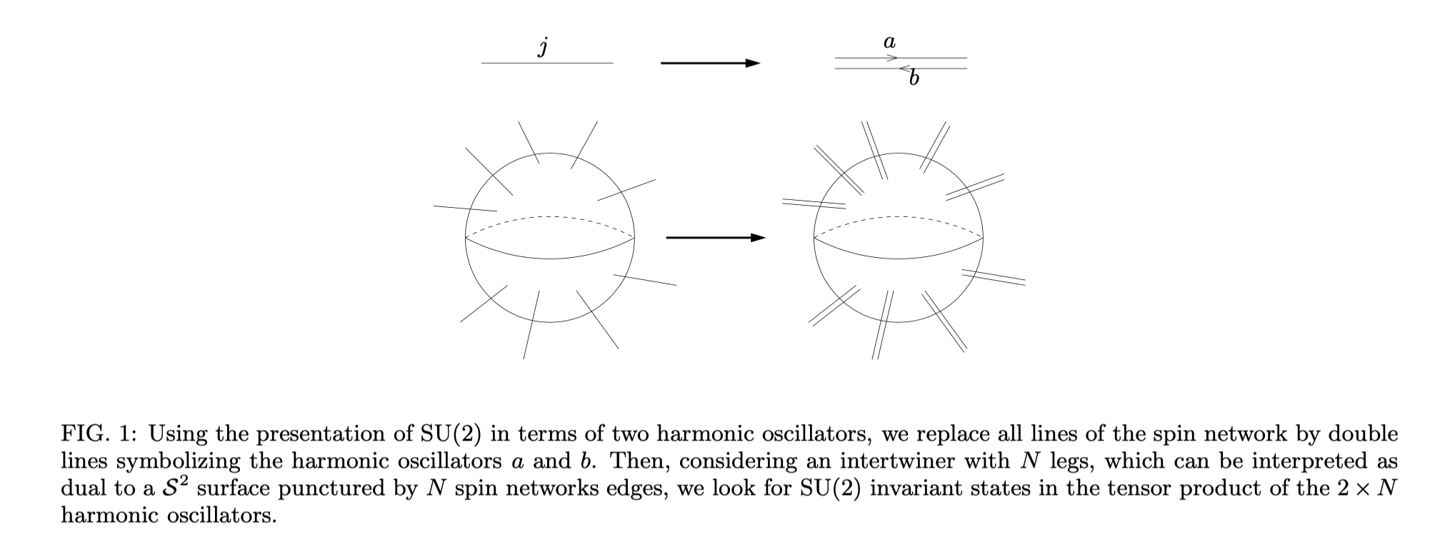
Finally, suppose we wanted to consider quantizing some arbitrary polyhedron. There's a difficulty with the representation above, which is that each face has one fixed $j$ value which doesn't change. Given some arbitrary classical polyhedron, who knows what conjuction of spins will match the areas? But it would be nice to have a way of quantizing arbitary polyhedra directly.
Looking ahead, we'll find that the states of two quantum harmonic oscillators can be used to represent a quantum spin with a variable $j$ value: in other words, we can treat the two oscillators as being in general a superposition of spins with all possible $j$'s. We can employ this representation for our polyhedra: each edge, instead of carrying a specific spin-$j$, now carries two harmonic oscillators, and each interaction vertex consists of $2n$ oscillators. We can then quantize a more or less arbitrary classical polyhedron without worrying about which exact spins to use for areas. And our unitary evolution explores the space of polyhedra where the area of the faces can change! Check out osc_quantum_polyhedron.py. It also turns out that this representation is particularly useful when it comes to constructing the "holonomy operators," which are associated to loops, act across vertices, and whose eigenvalues diagnose curvature.