As if inevitably, the dialectic carries on. If we can iterate counting up to get addition, we should be able to iterate addition to get: multiplication, whose "all-at-once" inverse is division. And just as before, we graduate to a new notion of number, a new interpretation of atoms: the rational numbers, which can be regarded as "piles of piles." Here's how it works.
If we have two piles of pebbles $A$ and $B$, we can multiply them by iterating the addition of $A$ by the number of pebbles in $B$, or vice versa.
$ \Large \{ \Large\bullet, \Large\bullet \} \times \Large \{ \Large\bullet, \Large\bullet, \Large\bullet \} = \Large \{ \Large\bullet, \Large\bullet \} + \Large \{ \Large\bullet, \Large\bullet \} + \Large \{ \Large\bullet, \Large\bullet \} = \Large \{ \Large\bullet, \Large\bullet, \Large\bullet \} + \Large \{ \Large\bullet, \Large\bullet, \Large\bullet \} $
$ \Large \{ \Large\bullet, \Large\bullet \} \times \Large \{ \Large\bullet, \Large\bullet, \Large\bullet \} = \Large \{ \Large\bullet, \Large\bullet, \Large\bullet, \Large\bullet, \Large\bullet, \Large\bullet \} $
$ 2 \times 3 = 3 \times 2 = 6 $
If we wanted we could display the last identity like this:
$ 2 \times 3 = 3 \times 2 = \begin{matrix} \Large\bullet & \Large\bullet \\\ \Large\bullet & \Large\bullet \\\ \Large\bullet & \Large\bullet \end{matrix} = \begin{matrix} \Large\bullet & \Large\bullet & \Large\bullet \\\ \Large\bullet & \Large\bullet & \Large\bullet \end{matrix} $
And correspondingly: $\frac{6}{3} = 2 $ and $ \frac{6}{2} = 3$. And we have it that $\frac{n}{1} = n$ for any $n$.
Now an important structure arises out of the interplay between addition and multiplication: the prime numbers. A prime number is a number than is only divisible by itself or $1$. Whereas $12$ could be expressed $2 \times 2 \times 3$, $7$ is just $7 \times 1$. The primes go like: $2, 3, 5, 7, 11, 13, 17, 19, \dots$ And in fact, there are an infinite number of primes. The proof goes back at least to Euclid.
First we observe, that every 2nd number is divisible by 2, every 3rd number is divisible by 3, every 4th number is divisible by 4, every 5th number is divisible by 5, and so on. It follows that if we add $1$ to any number, it won't be divisible by any of its old primes. For example, $14 = 2 \times 7$, but $15 = 3 \times 5$. If we think about it "musically," $14$ falls on the beat of $2$ and $7$: as I say, every 2nd number is divisible by $2$, every 7th number is divisible by $7$, and both beats fall on $14$. But if we add $1$ to $14$, it can't fall on the $2$-beat nor the $7$-beat, and this is a general rule.
$ 1 \mid \color{green}2 \mid \color{blue}3 \mid \color{green}2 \times \color{green}2 \mid \color{orange}5 \mid \color{green}2 \times \color{blue}3 \mid \color{purple}7\mid \color{green}2 \times \color{green}2 \times \color{green}2 \mid \color{blue}3 \times \color{blue}3 \mid \color{green}2 \times \color{orange}5 \mid \color{pink}{11}\mid \color{green}2 \times \color{green}2 \times \color{blue}3 \dots $
So suppose there were a largest prime number. We could then take that prime and all the prime numbers lower than the largest, multiply them all together and add $1$: this number couldn't be divisible by any of our known primes! And so, it must contain a yet larger prime within it. Hence, our initial assumption has led to a contradiction: therefore, the converse is true: there are an infinite number of prime numbers.
Now it is a fact that every counting number can be broken down uniquely into a product of primes. Which suggests the following idea. What if we introduce now an infinite number of colored pebbles, one for each prime? Under the hood, each will be just a pile of pebbles in disguise.
$ 1 \rightarrow \Large{\color{black} \bullet} \rightarrow \{ \Large\bullet \}$
$ 2 \rightarrow \Large{\color{green} \bullet} \rightarrow \{ \Large\bullet, \Large\bullet \}$
$ 3 \rightarrow \Large{\color{blue} \bullet} \rightarrow \{ \Large\bullet, \Large\bullet, \Large\bullet \}$
$ 5 \rightarrow \Large{\color{orange} \bullet} \rightarrow \{ \Large\bullet, \Large\bullet, \Large\bullet, \Large\bullet, \Large\bullet \}$
$ 7 \rightarrow \Large{\color{purple} \bullet} \rightarrow \{ \Large\bullet, \Large\bullet, \Large\bullet, \Large\bullet, \Large\bullet, \Large\bullet, \Large\bullet \}$
$ 11 \rightarrow \Large{\color{pink} \bullet} \rightarrow \{ \Large\bullet, \Large\bullet, \Large\bullet, \Large\bullet, \Large\bullet, \Large\bullet, \Large\bullet, \Large\bullet, \Large\bullet, \Large\bullet, \Large\bullet \}$
We could now write $12$ like this:
$ 12 = 2 \times 2 \times 3 = \Large\{ \Large{\color{green} \bullet}, \Large{\color{green} \bullet}, \Large{\color{blue} \bullet} \} = \Large\{ \{ \Large\bullet, \Large\bullet \}, \{ \Large\bullet, \Large\bullet \}, \{ \Large\bullet, \Large\bullet, \Large\bullet \} \} = \{ \Large\bullet, \Large\bullet, \Large\bullet, \Large\bullet, \Large\bullet, \Large\bullet, \Large\bullet, \Large\bullet, \Large\bullet, \Large\bullet, \Large\bullet, \Large\bullet \}$
So we have a new kind of pile: a pile of prime numbers. And the rule is: we multiply elements in a pile of primes together into a composite. Just as pebbles coexist "unordered" in an "additive pile," prime pebbles coexist "unordered" in a "multiplicative pile." At this level, the primes are our new atoms and we interpret "piles of piles" multiplicatively. We can have, of course, multiple "piles of piles" and we can combine them just like piles:
$ \Large\{ \Large{\color{green} \bullet}, \Large{\color{green} \bullet} \Large\} \times \Large\{ \Large{\color{orange} \bullet} \} \rightarrow \Large\{ \Large{\color{green} \bullet}, \Large{\color{green} \bullet}, \Large{\color{orange} \bullet} \Large\}$
$ 4 \times 5 = 20$
But what happens if we do something crazy like $\frac{3}{2}$? There's no counting number $n$ such that $n \times 2 = 3$. But if we can multiply, we must be able to divide. So again we have to introduce a new kind of number: a rational number. We just interpret $\frac{3}{2}$ as a fraction. We could think of this like introducing a little inverse pebble for each prime.
$ \frac{1}{1} \rightarrow \bar{\Large{\color{black} \bullet}}$
$ \frac{1}{2} \rightarrow \bar{\Large{\color{green} \bullet}}$
$ \frac{1}{3} \rightarrow \bar{\Large{\color{blue} \bullet}}$
$ \frac{1}{5} \rightarrow \bar{\Large{\color{orange} \bullet}}$
$ \frac{1}{7} \rightarrow \bar{\Large{\color{purple} \bullet}}$
$ \frac{1}{11} \rightarrow \bar{\Large{\color{pink} \bullet}}$
And the rule is that:
$\Large\{ \Large{\color{green} \bullet}, \bar{\Large{\color{green} \bullet}} \Large\} \rightarrow \Large\{ \Large{\color{black} \bullet} \Large\}$
$ 2 \times \frac{1}{2} = 1$.
If a prime pebble and its inverse appear in a pile together, we can remove them both: which is the same as replacing them with a $1$ pebble. And actually we can add as many $1$ pebbles as we please without changing the number represented by the pile. Moreover, we can add any number of pairs of primes and inverses, and our pile will still represent the same number. Once all the cancellations have taken place, we say we've reduced the rational number to "lowest terms."
We can take advantage of this freedom to add rational numbers. First, we have to find a common denominator, and then we can add the numerators without trouble.
$ \frac{1}{5} + \frac{2}{3} = \frac{3}{15} + \frac{10}{15} = \frac{13}{15} $
Finally, we also have our $-1$ pebble: $\Large{\color{red} \bullet}$, which can make piles negative. We can toss pairs of these pebbles into any multiplicative pile without changing the number represented.
$ \Large{\color{black} \bullet} \times \Large{\color{red} \bullet} = \Large{\color{red} \bullet}$
$ \Large{\color{red} \bullet} \times \Large{\color{red} \bullet} = \Large{\color{black} \bullet}$
If integers can keep track of credits and debts, which is related to the ability to arbitrarily decide what to regard as "0", rational numbers can keep track of different denominations, which is related to the ability to arbitrarily decide what to regard as "1".
For instance, maybe I have a ruler $A$ and I measure something to be $3$ units. You have a ruler $B$, and each unit of your ruler is worth two of mine: $\frac{yours}{mine}$. We could describe the relationship between our rulers with a rational number: $\frac{1}{2}$. So you would measure the same object to be $3 \times \frac{1}{2}$ or $\frac{3}{2}$ in your units. So rational numbers allow us to switch between different "currencies": it provides the exchange rate from gold to silver, dollars to cents, hours to minutes. Indeed, we recognize that if we want to communicate a number, in general we need to provide more context since we could be using different units to measure our numbers: we need to agree on how much of your "1" there is per my "1".
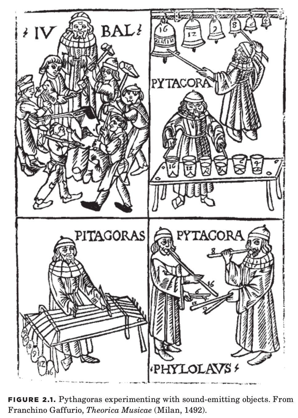
We can't help but mention the myths of Pythagoras, who believed that ratios governed the world. Ratios can represent rates. For example, velocity is the ratio between distance traveled and time past. Frequency is the ratio between the number of crests of a wave and an interval of time or space. Every $\frac{1}{52}$ years a week passes, about $7$ revolutions of the sun in the sky, or some more obscure planet.
The legend goes that in ancient times Pythagoras investigated the mathematics of a plucked string. Consider a guitar string, tightened over a soundboard. Pluck it and it produces a tone. Hold a note at the 12th fret, in other words: divide the string by $2$. You hear a tone with twice the frequency, called an octave higher.
$ frequency \approx \frac{1}{length} $
If I hold a note at the 7th fret, I've divided the string into $\frac{3}{2}$, and so I hear $\frac{2}{3}$ times the old frequency, a major fifth. If I hold a note at the 5th fret, I've divided the string into $\frac{4}{3}$, and so I hear a note $\frac{3}{4}$ lower. If I hold a note at the 4th fret, I've divided the string into $\frac{5}{4}$, and so hear a note $\frac{4}{5}$ lower, which is a major third. And now we have enough notes for a major chord. $\frac{1}{2} \frac{2}{3} \frac{3}{4} \frac{4}{5}$. We've only used the first three primes $2, 3, 5$ and found the tones most pleasing to harmonize against the base note. Strings whose lengths are related by the simple low integer ratios, when plucked together, harmonize. Divide the string by a more complicated fraction, the more dissonant the resulting note sounds with the base note. And so, Pythagoras developed a theory of music, about which notes to play, which divisions of the string to make: and the idea was that the ratios between the notes would be these simple ones.
We'll now go on a slight digression, for the sake of illustration. It's clear that when we hear a musical chord, we can distinguish the notes within it. Just like you can decompose a composite number into its primes, you can decompose a musical chord into its constituent notes. The idea is that there are an array of little bones in your ear, each of different length, and so when a sound wave hits the bones, different bones vibrate sympathetically to the different tones in the sound, which is then translated into neural pulses, etc. [I stand corrected! cf. How Do We Hear?. But the moral of the story is the same.] What you are doing is something called a Fourier transform. It turns out that any periodic signal can be decomposed into a sum of "sine waves" at frequencies $1, 2, 3, \dots$, each with a certain amplitude or loudness, and possibly phase shifted.
In other words, the simplest kind of tone is a "sine wave," or an oscillation at a fixed frequency, amplitude, and phase. Frequency tells you which note it is, amplitude tells you how loud it is, and phase tells you at what point in its oscillation, its vibration of the air, did the wave hit your ear. If we want more than one tone, we just add the waves on top of each other, superimposing them. We superimpose the waves, but of course: we hear the notes within it, the frequencies (meaning we have to listen for a certain amount of time to make out the note with certainty). Again, we'll come back to this, including what a "sine" is later. (Ps. check out audio.py to play around with a frequency analyzer!)
Anyway, let's hear some ratios:
import numpy as np
from IPython.display import (Audio, display)

def note(frequency=440., amplitude=500., phase=0, duration=1.0, rate=44100):
    t = np.linspace(0, duration, int(duration*rate))
    return amplitude*np.sin(2*np.pi*frequency*t + phase)

def chord(notes):
    max_length = 0
    for note in notes:
        if len(note) > max_length:
            max_length = len(note)
    resized_notes = []
    for note in notes:
        resized_note = note.copy()
        resized_note.resize(max_length)
        resized_notes.append(resized_note)
    return sum(resized_notes)

def melody(notes):
    return np.concatenate(notes)

def sing(song, rate=44100):
    display(Audio(song, rate=rate, autoplay=False))
    #import scipy
    #scipy.io.wavfile.write("song.wav", rate, song.astype(np.int16))

A = note(frequency=440,\
          amplitude=500,\
          phase=0,\
          duration=1,\
          rate=44100)

Db = note(frequency=440*(5./4.),\
          amplitude=500,\
          phase=0,\
          duration=1,\
          rate=44100)

E = note(frequency=440*(3./2.),\
          amplitude=500,\
          phase=0,\
          duration=1,\
          rate=44100)

sing(chord([A, Db, E]), rate=44100)
Sounds kinda funny.
An actual vibrating string, like on a violin, a guitar, or in a piano, actually vibrates as several frequencies at once. Imagine the string being plucked and vibrations being sent out from the place where you pluck it to the ends. The waves bounces back and forth between the two end points, and pretty soon, the whole string is only vibrating at frequencies where the number of crests of the wave can fit on the string.
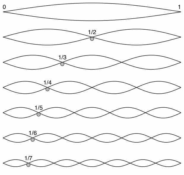
So the whole string can wiggle back and forth, then the left and the right half can wiggle with a "node" of stillness in the middle. And then you can have three crests, four, etc. You hear all the frequencies at once, with different amplitudes depending on the kind of string, the kind of resonator used, etc, which give the instrument its timbre. As time goes on, if there's damping, just as a spinning penny eventually vibrates rapidly as it finally comes to rest, the quieter, but higher frequency "modes" persist on the string, as the sound trails off into high pitched infinity.
def harmonics(max_harmonics=12, base_frequency=220., base_amplitude=100, duration=1.0):
    sing(melody([chord([note(frequency=base_frequency*j,\
                             amplitude=base_amplitude/j,\
                             duration=duration) for j in range(1, i+1)])\
                               for i in range(1, max_harmonics+1)]))
harmonics(max_harmonics=12,\
          base_frequency=220,\
          base_amplitude=100,\
          duration=1.0)
One can derive all this from the wave equation of the string, which is a partial differential equation.
$ \frac{d^{2}\psi(x, t)}{dx^2} = \frac{d^{2}\psi(x, t)}{dt^2}$.
Just for fun:
We separate independent variables, rewriting $\psi(x, t)$ as $\phi(x)\beta(t)$, obtaining:
$ \phi^{\prime\prime}(x)\beta(t) = \phi(x)\beta^{\prime\prime}(t) $
Dividing by $\phi(x)\beta(t)$, and we obtain all the x's and t's on separate sides of the equation, and equate them via $\lambda$.
$ \frac{\phi^{\prime\prime}(x)}{\phi(x)} = \frac{\beta^{\prime\prime}(t)}{\beta(t)} = -\lambda$
We then have two coupled ordinary differential equations:
$ \phi^{\prime\prime}(x) + \lambda\phi(x) = 0$ and $\beta^{\prime\prime}(t) + \lambda\beta(t) = 0$.
Suppose the string is of length 1, and fixed at $x=0$ and $x=1$.
$ \psi(0, t) = 0$ and $\psi(1, t) = 0$, so that $\phi(0) = 0$ and $\phi(1) = 0$.
It turns out that $\phi^{\prime\prime}(x) + \lambda\phi(x) = 0$ has an infinite number of solutions compatible with these boundary conditions, one for each of a countable infinitude of $\lambda_{n}$'s, where $\lambda_{n} = (n\pi)^{2}$, called "eigenvalues," each with an associated "eigenfunction" $\phi_{n}(x) = sin(\sqrt{\lambda_{n}}x) = sin(n\pi x)$, where $n = 1, 2, 3, \dots$. These are our sine waves, and they each satisfy the differential equation, and arbitrary sums of them also satisfy the differential equation. The counting numbers appear here because of the boundary conditions on the string. The frequency of each wave is $n\pi$. We can watch how the wave changes in time by substituting $\beta_{n}^{\prime\prime}(t) + \lambda_{n}\beta(t) = 0$ to get the time dependency. Maybe we add a damping term, some special initial condition, specify a coefficient for the tension of the string (you have to apply 4 times the tension to double the frequency), and so forth. We'll return here in the end as in quantum mechanics the idea of these vibratory "normal modes" will experience a vast generalization...
But before we go, I have to say: that last fact about tension was known to Pythagoras and actually Newton claims it was his actual inspiration for his law of gravity (he actually thought that perhaps the Pythagorans had known about gravity's "musical law" and kept it as an esoteric secret). One imagines the planets attached by strings. Newton says that $F=ma$ and $F_{gravity} = \frac{m_{1}m_{2}}{d^{2}}$, so that for the first mass: $\frac{m_{1}m_{2}}{d^{2}} = m_{1}a_{1}$, or $a_{1} = \frac{m_{2}}{d^2}$. You get the same acceleration if you either: half the distance (which gives a "note" twice as high) or multiply the the mass (or tension) by four. It's just like $f = \frac{\sqrt{tension}}{length}$. Acceleration is frequency squared? Of course, Netwon gave other more public arguments: the weakness of gravity can be conceptualized as getting proportioned over the surface area of a sphere ($4\pi r^{2}$) whose radius is the distance. Indeed, Pythagoras's theorem is lurking here: we shall come to that in the next section.
For now, we remain with Pythagoras and his ratios, governing above and below, generating the harmony of the spheres (as referenced by Kepler, who discovered, in fact, that the planets move in ellipses).
In honor of the ancients, let's listen to what it sounds like to count. We're going to count up from 1, and at each counting number, we're going to break that number down into its primes. Suppose we're at $12 = 2 \times 2 \times 3$. For a moment, we'll hear a chord of three sine waves: a sine wave with frequency $2$, a sine wave with frequency $2$, and a sine wave of frequency $3$. In fact, this is the same as a sine wave with frequency $2$ and amplitude $2$ and a sine wave of frequency $3$ (amplitude $1$). In other words, we'll convert each counting number into a chord of sine waves, a sine wave for each prime in the decomposition with a loudness proportional to the number of each prime. Every second beat, therefore, is an octave; every third, a fifth, and so on, forever, every possible rhythm and harmony overlaid.
import numpy as np
from IPython.display import (Audio, display)

def note(frequency=440., amplitude=500., phase=0, duration=1.0, rate=44100):
    t = np.linspace(0, duration, int(duration*rate))
    return amplitude*np.sin(2*np.pi*frequency*t + phase)

def chord(notes):
    max_length = 0
    for note in notes:
        if len(note) > max_length:
            max_length = len(note)
    resized_notes = []
    for note in notes:
        resized_note = note.copy()
        resized_note.resize(max_length)
        resized_notes.append(resized_note)
    return sum(resized_notes)

def melody(notes):
    return np.concatenate(notes)

def sing(song, rate=44100):
    display(Audio(song, rate=rate, autoplay=False))
    #import scipy
    #scipy.io.wavfile.write("song.wav", rate, song.astype(np.int16))

########################################################################

def factorize(n):
    factors = []
    d = 2
    while d*d <= n:
        while (n % d) == 0:
            factors.append(d)
            n //= d
        d += 1
    if n > 1:
        factors.append(n)
    return factors

########################################################################

def counting_music(count_max=100, base_frequency=220, base_amplitude=100, chord_duration=0.5):
    sing(melody([chord([note(frequency=base_frequency*factor,\
                             amplitude=base_amplitude,\
                             duration=chord_duration) for factor in factorize(i)+[1]])\
                               for i in range(1, count_max)]))
counting_music(count_max=200,\
               base_frequency=220,\
               base_amplitude=100,\
               chord_duration=0.4)
Here's an observartion. If we consider just the cycles originated by the primes: every $2$, every $3$, every $5$, every $7$, every $11$, every $13$, etc, we notice that each new prime has to fall in the gaps left over in between the cycles of the previous primes.
At first the primes come fast, but soon they slow down and get more spaced out. But despite this general observation, the individual location of each prime number, or the spacing in between adjacent primes, is difficult to predict: in the worst case, if you're counting, to know if the next number is prime or not, you have to go back to the beginning and make your $2$-cycles and $3$-cycles and $5$-cycles, and see if the next number falls on the beat of prime, or if there's a gap waiting for a new prime to fill it. Despite the simplicity and regularity of the rhythm of every two, every three, every five, etc, each new prime comes as a suprise, as if by chance. And there's been a great effort extended to quantify the statistical randomness of the primes, centering around a conjecture known as the Riemann Hypothesis. And there's the famous Prime Number Theorem, which says basically that for large $N$, the probability that a random number is prime is about $\frac{1}{ln(N)}$.
But what's clear from the above is that there is a kind of complementarity between addition and multiplication: if you give me the magnitude, I have to do some work to figure out the primes; if you give me primes, I have to do some work to figure out the magnitude. Now it happens that it's way easier to multiply than to decompose into primes, an asymmetry which is the basis of certain crypotographic systems.
Finally, there remains a question about $0$. What happens if we take $\frac{1}{0}$? If we want to be able to add, subtract, multiply, and divide all our numbers, we need to find an interpretation of this. (This assumes we've added new kind of pebble for $0$, which must have an inverse.) So we actually need one last number.
We say: $\frac{1}{0} \rightarrow \infty$ and $\frac{1}{\infty} = 0$. But if that's the case, then $-\frac{1}{\infty}$ must also be $0$ since $-0 = 0$. So we have the idea of identifying positive and negative $\infty$.
Here's one way to think of this:
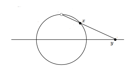
The idea is imagine all the rational numbers except $\infty$ arranged on a line. This can be done because every rational number divides the rationals into those less than and those greater than it. We then imagine a point at infinity beyond all the points on the left, and a point at infinity beyond all the points on the right, and we say that it's the same infinity. What we've done is wrap up the number line into a circle. Every rational number can be uniquely mapped to the circle via this "stereographic projection".
There's another way to think about this. We can think about a rational number as a division of a pie.
Consider that we can represent a location on a two dimensional plane if we fix two lines at right angles: the x-axis and the y-axis. The coordinates $(x, y)$ represent: go horizontally by x and vertically by y, starting from $(0,0)$. Then you'll arrive at the desired location.
You may recall that we can represent a line in a plane with an equation $y = mx + b$, where b represents where the line intersects the y-axis, and $m$ is the slope of the line. It's a ratio: $m = \frac{rise}{run} = \frac{\Delta y}{\Delta x}$. Suppose the line goes thru the origin. Then our line is just $y = mx$. By choosing different values for $m$, we can explore all the lines through the origin, except for one: what about a completely vertical line? The equation is just $x = 0$. Given just $y = mx$, this would mean that $y = 0$ as well, but we know that's not the case: we want all the points with $x = 0$ where y can be anything at all. What's worse, we look at the slope $\frac{rise}{run} = \frac{1}{0}$! So what can we do?
In short, we've noted that we can associate every rational number to a line through the origin on a plane except for one: a vertical line. So we add to the rationals one extra number, $\infty$. In doing so, we form a "projective space," and identify the rational numbers (plus $\infty$) with lines through the origin in two dimensions. If we put a circle of some size centered at the origin, we notice that every line intersects the circle twice: so the "rational projective line" is also just a circle with antipodal points identified: it is the space of ratios, of slopes.
Consider that given some random line in the plane $y = mx + b$, our lines through the origin will each intersect that line in one place, all except for one: the line through the origin parallel to it. We say that line intersects our given line "at $\infty$", and the missing intersection point lives there. Parallel lines are just lines that intersect at infinity in a projective space! You can think of it like: it turns out the two lines are just part of one really big circle.
There's an easy way to represent this. Suppose instead of writing a rational number as $\frac{2}{3}$, we write it as $\begin{pmatrix} 3 \\ 2 \end{pmatrix}$, where we swap x and y inspired by $\begin{pmatrix} \Delta_{rise} \\ \Delta_{run} \end{pmatrix}$.
Actually, we can represent it as any $a \times \begin{pmatrix} 3 \\ 2 \end{pmatrix}$, where we multiply each element in the list by $a$, because to recover a fraction from $\begin{pmatrix} y \\ x \end{pmatrix}$, we'll take $\frac{x}{y}$. Clearly $\begin{pmatrix} a \times y \\ a \times x \end{pmatrix} \rightarrow \frac{a \times x}{a \times y} = \frac{x}{y}$.
So we have two coordinates, but they only represent the point up to multiplication by any number.
In a sense, we're taking into account that the fraction might not be in lowest terms. Say we have $\frac{12}{3}$. We could write it as: $ \begin{pmatrix} 3 \\ 12 \end{pmatrix}$, which is just $ 3 \times \begin{pmatrix}1 \\ 4 \end{pmatrix} $, because it's the same as $\frac{4}{1}$. Note that you can always put $\begin{pmatrix} y \\ x \end{pmatrix}$ into the standard form $\begin{pmatrix} 1 \\ \frac{x}{y} \end{pmatrix}$--but for one exception.
If we have $\frac{\Delta_{rise}}{\Delta_{run}} = \frac{0}{1}$, we get $\begin{pmatrix} 1 \\ 0 \end{pmatrix}$. But if we have $\frac{\Delta_{rise}}{\Delta_{run}} = \frac{1}{0}$, we get $\begin{pmatrix} 0 \\ 1 \end{pmatrix}$, which is a projective representation of our equation $x=0$. And we take $\begin{pmatrix} 0 \\ 1 \end{pmatrix}$ to correspond to a point at $\infty$.
This causes no interpretative difficulties: if we run into an infinity, it's just a "vertical line": and then, we can just turn our head sideways, flip $\begin{pmatrix} 0 \\ 1 \end{pmatrix}$ into $\begin{pmatrix} 1 \\ 0 \end{pmatrix}$, horizontal into vertical, and there's no problem.