I want to give you a visceral sense of what entanglement is, really concretely. We're going to consider a case where entanglement can be understood in relatively simple geometric terms. We're going to start in a seemingly very specific place in our discussion of the very general phenomenon of entanglement: the sphere. And we'll see what can generalize from there.
So the story begins with the sphere.
As you probably know, the sphere can be defined with the following equation:
$ r^{2} = x^{2} + y^{2} + z^{2} $
Here $r$ is the radius of the sphere. We recognize that $ \sqrt{x^{2} + y^{2} + z^{2}} $ is the length of the vector from the origin to the point $ (x, y, z) $. So this equation is true for all points of constant radius from the origin in three dimensions: in other words, a sphere.
But we're too cool for that so we like to represent points on our sphere using complex numbers. First, we pick a north pole/south pole axis. Then we do the stereographic projection from the sphere to the complex plane, taken to be an infinite plane cutting the sphere at its equator. All the points on the sphere save one are projected to a unique location on the plane and so can be written as a complex number $ x+iy$. All except the north pole, the point of projection, which we take to be a point beyond every point along the circular planar horizon, a point at infinity. So we map:
$ (x, y, z) \rightarrow \mathbb{C} + \infty $
But here's the thing: we need two "coordinate charts."
Suppose we have a function $f(x, y, z)$ and we want to instead use the $f( \mathbb{C} \ or \ \infty )$ version. Everything is fine until we try plugging infinity into whatever expression $ f $ is equal to: what do we do? Simple. We have two coordinate systems: one given by a projection from the north pole, and one given by a projection from the south pole. And if we worry about $ f_{north}(\infty) $, we just take $ f_{south}(0) $, and vice versa. Indeed, it's as much to say: as you move around the "Riemann sphere," if your coordinate systems moves with you, $ \infty $ is always the point antipodal to you; and so $ \infty $ acts as your "double," with a coordinate chart of its own, showing you at $ \infty $.
We're going to come back these two "coordinate charts" in a surprising way soon enough.
Next we have to talk about Mobius tranformations. They are the most natural thing in the $ \mathbb{C} + \infty $ world.
$ f(z) = \frac{az+b}{cz+d} $
where $ a, b, c, d $ satisfy $ ad - bc \neq 0 $. It's understood that the $ z $ can be a complex number or infinity, and if we need to evaluate at infinity we use our flipped coordinate chart.
We can comprehend a Mobius transformation completely geometrically as a generalization of the stereographic projection. Given the points on the complex plane, first stereographically project them to the unit sphere. Then you are allowed to translate the sphere and rotate it however you like in 3D, passing it above below the plane, who cares. And then at the end, project all the points back to the same plane.
These transformations are also known as "conformal transformations": they are 1-to-1, and they deform distances, but locally preserve angles. So that all right angles and all circles are preserved. The classic reference is:
If we get tired of the whole $ \mathbb{C} + \infty $ thing, we can always work with our friend the complex projective space.
$ \mathbb{C} + \infty \rightarrow \begin{pmatrix} \alpha \\ \beta \end{pmatrix} $
Where if you recall: some $ z \rightarrow \begin{pmatrix} z \\ 1 \end{pmatrix}$ (normalized) or $ \begin{pmatrix} 1 \\ 0 \end{pmatrix} $ if $ \infty $.
So we've traded our infinity for a second complex dimension. And now our (x, y, z) is encoded in our 2d complex projective vector up to multiplication by any (complex) scalar.
Well, you'll be pleased to know that we can upgrade our Mobius transformation is a very obvious way.
$f(z) = \frac{az+b}{cz+d} \Rightarrow \begin{pmatrix} a & b \\ c & d \end{pmatrix}$, with determinant equal to 1. These are called SL(2,$\mathbb{C}$) matrices.
Now this is a "matrix" group and we've seen it before. It has six "generators" which are just two copies of the 3 Pauli matrices, the second set of 3 being multiplied by i.
$ SL(2,\mathbb{C}) = e^{(a+bi)X + (c+di)Y + (e+fi)Z} $
If we use only complex components, we get a subgroup SU(2), corresponding to the (double cover) of 3D rotations. And if we use real components too, we get also "boosts".
This is already starting to sound like relativity.
Suppose we have a point on the unit sphere. We could write it as a 4-vector:
$0 = 1 - x^{2} - y^{2} - z^{2} \rightarrow (1, x, y, z) $
If, for example, we're working in the complex projective space, with a qubit, where we've taken the normalization of our state to be 1, we could form:
$ \begin{pmatrix} t \\ x \\ y \\ z \end{pmatrix} = \begin{pmatrix} \langle \psi \mid \psi \rangle \\ \langle \psi \mid X \mid \psi \rangle \\ \langle \psi \mid Y \mid \psi \rangle \\ \langle \psi \mid Z \mid \psi \rangle \\ \end{pmatrix} $
One can show that the 4-vector asociated to a qubit transforming under $SL(2, \mathbb{C})$ transforms under a Lorentz transformation. In other words, a transformation that preserves: $ t^{2} - x^{2} - y^{2} - z^{2} $. These are the transformations in special relativity that take you to boosted and rotated reference frames. The 4-vector could represent the Minkowski space position of a particle $(t, x, y, z)$, or it could represent its momentum $(E, P_{x}, P_{y}, P_{z})$, where E is the energy and the P's are the momentum in the X, Y, and Z directions. More on this in a moment.
We can see the correspondence plainly in the following way.
Suppose we have a 4-vector $ (t, x, y, z) $. We can uniquely associate it to a Hermitian matrix like so:
$$ H = tI + xX + yY + zZ = t\begin{pmatrix}1 & 0 \\ 0 & 1 \end{pmatrix} + x\begin{pmatrix} 0 & 1 \\ 1 & 0 \end{pmatrix} + y\begin{pmatrix}0 & -i \\ i & 0 \end{pmatrix} + z\begin{pmatrix} 1 & 0 \\ 0 & -1 \end{pmatrix} = \begin{pmatrix} t + z & x - iy \\ x + iy & t - z \end{pmatrix}$$import numpy as np
import qutip as qt
IXYZ = {"I": qt.identity(2),\
"X": qt.sigmax(),\
"Y": qt.sigmay(),\
"Z": qt.sigmaz()}
a = qt.rand_ket(2)
# normalized qubit -> 4 vector
a4 = np.array([qt.expect(IXYZ[o], a) for o in ["I", "X", "Y", "Z"]])
# 4-vector -> hermitian matrix
# note in real life: a factor of 1/2
h = sum([a4[i]*IXYZ[o]/2 for i, o in enumerate(["I", "X", "Y", "Z"])])
# hermitian matrix -> 4-vector
h4 = np.array([qt.expect(IXYZ[o], h) for o in ["I", "X", "Y", "Z"]])
print((np.isclose(a4,h4)).all())
print(h == a*a.dag())
If we have a qubit $ \mid \psi \rangle $, what we did above amounts to taking $ \mid \psi \rangle \langle \psi \mid $.
We can transform hermitian matrices with $SL(2, \mathbb{C})$ by acting on them from both sides.
$ H \rightarrow UXU^{\dagger} $
What do we know about these $ U $ matrices? Their determinant is equal to 1. This means that as linear transformations they preserve the determinant of matrices they act on. What's the determinant of our of our 2x2 hermitians?
$ \begin{vmatrix} t + z & x - iy \\ x + iy & t - z \end{vmatrix} = (t + z)(t - z) - (x + iy)(x - iy) = t^{2} - z^{2} - x^{2} - y^{2} $
In other words, the determinant of the hermitian matrix is just the Lorentz norm of its corresponding 4-vector. Since $SL(2, \mathbb{C})$ matrices preserve the determinant they therefore fully represent Lorentz transformations.
Now here's an interesting fact: if, as we've seen, a hermitian matrix can be written as an outer product for some $ \psi $, as $ \mid \psi \rangle \langle \psi \mid $, then: it represents a pure state, and its (x, y, z) point lies on the sphere $ t^{2} = x^{2} + y^{2} + z^{2} $ or $ E^{2} = P_{x}^{2} + P_{y}^{2} + P_{z}^{2} $ if we're working with momenta. Now this is the unit sphere if we're working with normalized states in quantum mechanics. But let's allow the state to have arbitrary norm. Then in special relativity, the corresponding 4-vector would represent the momentum of a massless particle:
$ E^{2} - P_{x}^{2} - P{y}^{2} - P_{z}^{2} = m^{2} $ for $m = 0$.
And we can interpret this as a photon rushing in or out with a certain color (frequency proportional to energy) in a certain direction in 3D. The fact that a massless particle travels always at the speed of light corresponds to the fact that its 4-vector describes a point on the surface of its sphere. Picture its momentum like an arrow from the center of the sphere to that point: it can't go any faster, that's why the point lies on the surface.
But what if the particle does have a mass? Then it has to travel slower than the speed of light. And this corresponds to a hermitian matrix that can't be broken down into a single outer product, a rank-2 matrix, not a rank-1 matrix. And so it has to be written as a sum $a\mid \psi \rangle \langle \psi \mid + \ b\mid \phi \rangle \langle \phi \mid $. And in our representation, this corresponds to a point in the interior of the sphere.
Now when we're talking about quantum mechanics, this represents a general mixed state, or density matrix for a qubit. And incidentally, the rule for density matrices generally speaking is that their eigenvalues are all positive and when normalized sum to 1. And you can see that if you take the expectation values of the X, Y, Z operators for generally entangled qubits, the resulting points lie within the interior of the sphere, the maximally mixed state being in the center.
So on the one hand, we have the relativistic geometry of momentum space, which by the way, is the space we actually see around us on the "celestial sphere"; and on the other hand, we have the quantum geometry of the qubit, a little spin 1/2. And there is an intimate relationship. In what follows, we'll use the fact that it's easy to visualize relativity to visualize the quantum case.
(Incidentally, a word to the wise: one can really represent a lot of classical relativity theory in this way including the "little groups" of particles. For a massless particle, its hermitian matrices can be expressed as the outer product of a bra and a ket: now these each have an overall complex phase, and if we rotate each of them contrary to each other before we combine them, they will combine to give the same hermitian matrix as before. So the hermitian matrix is really only defined by the bra and the ket up to an arbitrary secret phase between the two parts. Correspondingly, the little group of a massless particle is U(1), the circle group. It's the photon corkscrewing in the plane orthogonal to its motion. And we can rotate the polarization of a photon without changing its momentum and vice versa. If we have a massive particle, we can break its hermitian matrix into four parts: a sum of two outer products. Now you could wonder: what could we do to these guys that doesn't change the Hermitian matrix they represents? It turns out to be (basically) SU(2): in other words, there's a qubit hidden inside there. We won't go into the details here, but similarly to before, you separate out two parts, and if you do a 3d rotation to the one, and the opposite rotation to the other, then the hermitian matrix everyone combines into is left invariant.)
This is the spin of a massive particle: the little group of a massive particle is SU(2): you can rotate its spin without changing the particle's momentum. But to expound on this would take us too far afield--we're only entering the territory to glean knowledge of quantum mechanical spins.
But before we go on, let's actually see it all happen. Let's simulate the relativistic photon sphere! We'll see the classic special effects including the blue shifting in the direction of mostion!
import qutip as qt
import numpy as np
import vpython as vp
scene = vp.canvas(background=vp.color.white)

def pure_to_four(pure):
    return np.array([qt.expect(qt.identity(2), pure),\
                     qt.expect(qt.sigmax(), pure),\
                     qt.expect(qt.sigmay(), pure),\
                     qt.expect(qt.sigmaz(), pure)])
n = 10
dt = 0.001
pts = [np.random.randn()*qt.rand_ket(2)/2 for i in range(n)]
mobius = sum([o*c for o, c in zip([qt.sigmax(), qt.sigmay(), qt.sigmaz()],\
                           dt*(np.random.randn(3)+1j*np.random.randn(3)))]).expm()
print(np.linalg.det(mobius.full()))

vsphere = vp.sphere(color=vp.color.blue, opacity=0.4)
vpts = [vp.sphere(radius=0.15, make_trail=True, emissive=True) for pt in pts]

for t in range(5000):
    for i in range(n):
        pts[i] = mobius*pts[i]
        txyz = pure_to_four(pts[i])
        vpts[i].pos = vp.vector(*txyz[1:]/txyz[0])
        vpts[i].color = vp.color.hsv_to_rgb(vp.vector(txyz[0] if txyz[0] < 0.6 else 0.6, 1,0.5))
        vp.rate(150)
Okay, so now comes the punchline. We can use all this machinery from classical relativity theory to visualize the entanglement between two qubits.
The idea is this: suppose we have two entangled qubits A and B. We want to visualize their entanglement. So we go through all the points on the surface of A's sphere, which correspond to all of A's pure states, and form the projectors onto those points. These are all the states A might end up in due to some measurement along some axis. We then see how B is "steered" due to that projection. Because of the entanglement, when A ends up in a certain state, it's as if a linear map is applied to B.
In other words, we can think of entanglement like a map from A to B (and vice versa). We form all possible projectors corresponding to points on the sphere and tensor them with the identity so they only act on A, say. And we project the entangled state using each projector in turn, and due to the entanglement B will be steered to a certain state. B's state will be weighted by the probability of the outcome for A, unless normalized.
To visualize this, we pepper A's sphere with points, each with a color unique to its location. We then project A into each of those states in turn, and see where B is projected to: we take B's X, Y, Z expectation values and place a star there for B which is the same color as A's star. And for now, let's not normalize the state afterwards.
import qutip as qt
import numpy as np
import vpython as vp
from itertools import product
scene = vp.canvas(background=vp.color.white)

#######################################

def normalize(v):
    n = np.linalg.norm(v)
    if n != 0:
        return v/n
    else:
        return v

def xyz_c(xyz, pole="south"):
    x, y, z = xyz
    if (pole=="south"):
        if np.isclose(z,-1):
            return float("Inf")
        else:
            return x/(1+z) + 1j*y/(1+z)
    elif (pole=="north"):
        if np.isclose(z,1):
            return float("Inf")
        else:
            return x/(1-z) + 1j*y/(1-z)

def c_spinor(c):
    if c == float('Inf'):
        return np.array([0,1])
    else:
        return normalize(np.array([1, c]))

def xyz_spinor(xyz):
    return c_spinor(xyz_c(xyz))

####################################################

vp.scene.width = 1000
vp.scene.height = 800

#state = qt.rand_ket(4)
state = qt.tensor(qt.rand_ket(2), qt.rand_ket(2))
#state = qt.bell_state("00")
state.dims = [[2,2],[1,1]]

N = 4
XYZs = []
Aprojectors = []
for x in np.linspace(-1,1,N):
    for y in np.linspace(-1,1,N):
        for z in np.linspace(-1,1,N):
            xyz = np.array([x,y,z])
            if(np.linalg.norm(xyz) > 0):
                xyz = xyz/np.linalg.norm(xyz)
                XYZs.append(xyz)
                spinor = qt.Qobj(xyz_spinor(xyz))
                proj = spinor*spinor.dag()
                Aprojectors.append(qt.tensor(proj, qt.identity(2)))

LXYZ = {"I": qt.tensor(qt.identity(2), qt.identity(2)),\
        "X": qt.tensor(qt.sigmax(), qt.identity(2)),\
        "Y": qt.tensor(qt.sigmay(), qt.identity(2)),\
        "Z": qt.tensor(qt.sigmaz(), qt.identity(2))}
RXYZ = {"I": qt.tensor(qt.identity(2), qt.identity(2)),\
        "X": qt.tensor(qt.identity(2), qt.sigmax()),\
        "Y": qt.tensor(qt.identity(2), qt.sigmay()),\
        "Z": qt.tensor(qt.identity(2), qt.sigmaz())}

vAsphere = vp.sphere(pos=vp.vector(-1.5,0,0),\
                     opacity=0.2, color=vp.color.blue)
vAarrow = vp.arrow(pos=vAsphere.pos)
vBsphere = vp.sphere(pos=vp.vector(1.5,0,0),\
                     opacity=0.2, color=vp.color.red)
vBarrow = vp.arrow(pos=vBsphere.pos)
vApts = [vp.sphere(radius=0.07,\
                    pos=vAsphere.pos+vp.vector(*xyz),\
                    color=vp.vector(*xyz))\
                        for i, xyz in enumerate(XYZs)]
vBpts = [vp.sphere(radius=0.07,\
                   color=vp.vector(*xyz))\
                           for i, xyz in enumerate(XYZs)]

def review(normalize=False):
    global state, XYZs, Aprojectors, LXYZ, RXYZ
    for i, xyz in enumerate(XYZs):
        b_state = (Aprojectors[i]*state).ptrace(1)
        b_xyz = np.array([qt.expect(qt.sigmax(), b_state),\
                           qt.expect(qt.sigmay(), b_state),\
                           qt.expect(qt.sigmaz(), b_state)])
        if normalize:
            b_xyz = b_xyz/np.linalg.norm(b_xyz)
        vBpts[i].pos = vBsphere.pos+vp.vector(*b_xyz)
    vAarrow.axis = vp.vector(qt.expect(LXYZ["X"], state),\
                             qt.expect(LXYZ["Y"], state),\
                             qt.expect(LXYZ["Z"], state))
    vBarrow.axis = vp.vector(qt.expect(RXYZ["X"], state),\
                             qt.expect(RXYZ["Y"], state),\
                             qt.expect(RXYZ["Z"], state))
    vp.rate(100)
review()
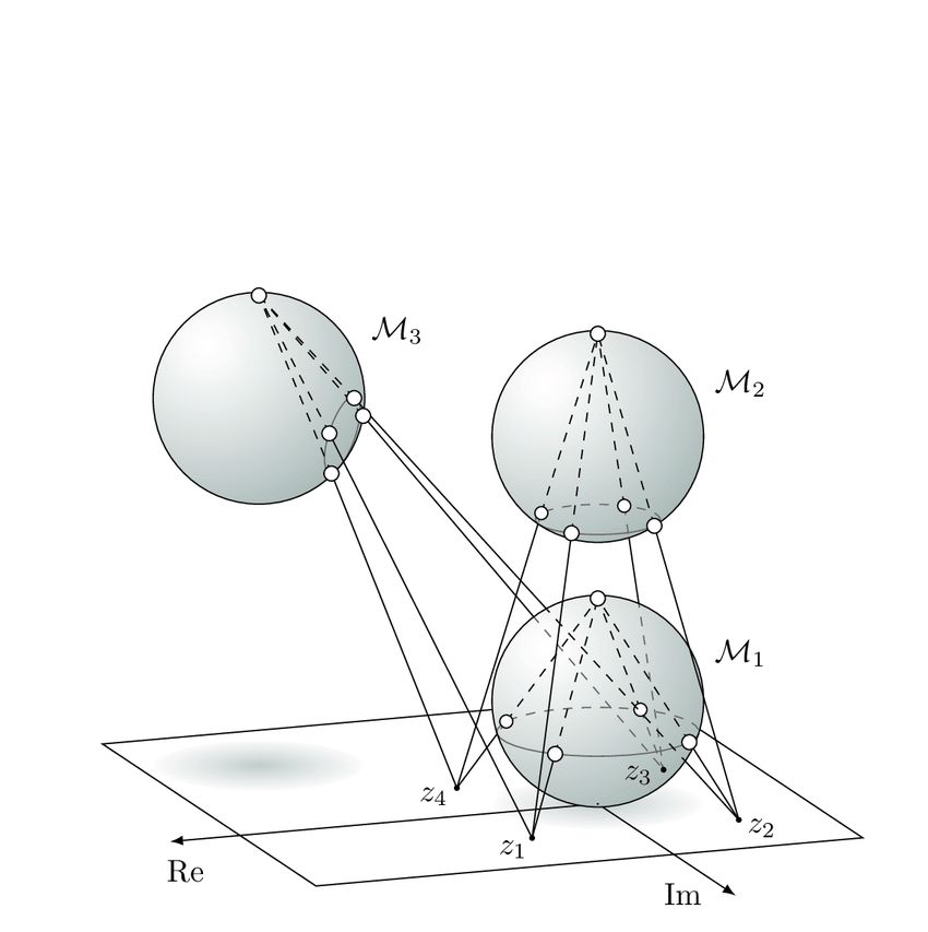
If we think of the entanglement between A and B as a map from A's sphere to B's sphere, then we can see that the image of A's sphere is an ellipsoid. In other words: a squished sphere oriented and placed within the unit sphere. Also shown are the expected values of A and B's spin axes. Cf. Quantum Steering Ellipsoids from Jetvic, Pusey, Jennings, et Rudolph for a similar construction.
Look at the three different cases. When A and B are separable, the ellipsoid reduces down to B's spin axis. In other words, no matter A's state, B ends up in the same state, which it's already in. So there's no correlation between them. When A and B are generally entangled, for each state A ends up in, B's spin axis gets steered to a corresponding location. But remember this spin axis is statistical, in a quantm mechanic sense. Despite steering, there is still quantum uncertainty w/r/t B's outcome, due to the fact that even if B's spin axis gets steered, one still has to choose a axis to measure along and the answer B gives will be probabilistic. Nonetheless, A can control the variation of B around its spin axis, and this is represented by the fatness of the ellipsoid. So fatter ellipsoids are more entangled.
Finally, consider the cup state, the maximally entangled state. A's sphere is mapped to another sphere! But it's flipped upside down along the Y axis. This is because the $ \mid 00 \rangle \ + \mid 11 \rangle $ state is entangled specifically in terms of the Z-basis. Now we note that under a Y flip, points on the equator are mapped to themselves. In other words, if we make a measurement on A along the Z axis, then B perfectly correlates with A. But notice that if A were measured along the Y axis, then B would anticorrelate with A.
Here's an interesting way to think about this. Recall before that we needed two coordinate charts to cover the Riemann sphere, one given by stereographic projection from the North Pole vs the South Pole. Well, that's just our Y flip! So when two qubits are maximally entangled we could actually view their spheres as two coordinate charts of the same sphere, the Riemann sphere!
And finally, the antisymmetric state leads to A and B having inverted spheres: because the overall angular momentum between them must be 0.
Finally, recall the meaning of the ellipsoid. Each point on A's sphere is mapped somewhere in B's sphere. And the depth of each point in B's sphere corresponds to the probability of the outcome for A. This is because when we do the projection onto A, we're throwing out some information, and so B is steered to a state in a certain direction, but the norm of that state depends on the probability of the original outcome for A. So deeper into the sphere means more improbable; and working outward, things become more probable, until certain when on the surface.
But when we measure one half of a pair of entangled particles, the two end up in a separable states. In other words, we end up with two separable pure states with a certain probability. So if we want literally the states B is steered to, we should normalize all the points, projecting them outward onto the surface of the sphere.
We're going to get something quite like a Mobius transformation from A's sphere to B's sphere. Imagine a sphere centered within a sphere. You could think of boosts as "squishing" the inside sphere orthogonal to the boost direction. But this wouldn't distinguish between opposite boost directions. So you could encode that in a translation of the ellipsoid within the outer sphere. A map outward from the inner ellipsoid to the outer sphere along projections from the center of the outer sphere would be 1-to-1 as long as the ellipsoid contained the center of the outer sphere and the ellipsoid wasn't a degenerate line, and I believe this map would be conformal-- although I'm not sure of the exact proof this. But what about the case of separable qubits? All points on A's sphere are mapped to the same point on B's sphere. This can't technically be a Mobius transformation since Mobius transformations are 1-to-1. Indeed, even if we boost a constellation so all its points are apparently coincident in the boost direction, they are really just ever more infinitesimally close to each other, since they angles between them are always preserved. But let's roll with it because it provides a nice analogy.
Indeed, this point of view, being entangled or not can be interpreted in terms of a relativistic analogy: separable states are states maximally boosted relative to each other, as if the particles were moving at the speed of light relative to each other; and at the other end of the spectrum, the maximally entangled states are as if the particles were at rest relative to each other. In other words, nature herself has given us a metaphor! Separable states are like two things moving at the speed of light relative to each other: no time to chat! Maximally entangled states are like two things at rest relative to each other.
And we can actually use this fact to our advantage. It turns out there's an easier way to calculate our ellipsoid.
Recall from our discussion of the Pauli basis that a 4x4 matrix can be expressed in terms of the matrix inner product with the following 16 matrices.
$$ \begin{matrix}II & IX & IY & IZ \\ XI & XX & XY & XZ \\ YI & YX & YY & YZ \\ ZI & ZX & ZY & ZZ\end{matrix} $$We can now see that this is nothing other than a generalization of our 4-vector formalism. Note that the 4-vectors of A and B are just the first row/column, and the ellipsoid is encoded in the 3x3 cross correlations.
So if we have a two qubit state $\mid AB \rangle$, we can form its density matrix and express it in the Pauli basis. Because density matrices are hermitian the resulting 4x4 matrix will be real valued.
Now suppose we have a qubit state $ \mid \psi \rangle $.
We can project A in $\mid AB \rangle$ into the $ \mid \psi \rangle $ state and look at the resulting partial state of B. This is a hermitian density matrix.
$$ \rho_{B} = \big( (\mid \psi \rangle \langle \psi \mid \otimes I)\mid AB \rangle \big)_{tr_{A}} $$We can expand it as a 4-vector:
$$ \rho_{B} \rightarrow \begin{pmatrix}I \\ X \\ Y \\ Z \end{pmatrix}_{\vec{\rho_{B}}} $$Now there's another way to get this same vector.
We expand out the qubit state we're using as a projector as a 4-vector:
$$ \mid \psi \rangle \rightarrow \begin{pmatrix}I \\ X \\ Y \\ Z \end{pmatrix}_{\vec{\mid \psi \rangle}} $$And we multiply by our 4x4 real DM in the Pauli basis:
$$ \begin{pmatrix}I \\ X \\ Y \\ Z \end{pmatrix}_{\vec{\mid \psi \rangle}}\begin{pmatrix}II & IX & IY & IZ \\ XI & XX & XY & XZ \\ YI & YX & YY & YZ \\ ZI & ZX & ZY & ZZ\end{pmatrix}_{\vec{\rho_{AB}}} = \begin{pmatrix}I \\ X \\ Y \\ Z \end{pmatrix}_{\vec{\rho_{B}}}$$And conversely:
$$ \begin{pmatrix}II & IX & IY & IZ \\ XI & XX & XY & XZ \\ YI & YX & YY & YZ \\ ZI & ZX & ZY & ZZ\end{pmatrix}_{\vec{\rho_{AB}}}\begin{pmatrix}I \\ X \\ Y \\ Z \end{pmatrix}_{\vec{\mid \psi \rangle}} = \begin{pmatrix}I \\ X \\ Y \\ Z \end{pmatrix}_{\vec{\rho_{A}}}$$And $ \vec{\rho_{AB}} $ changes under 4x4 Lorentz transformations on A and B separately like:
$ \vec{\rho_{AB}} \rightarrow \Lambda_{A} \vec{\rho_{AB}} \Lambda_{B}^{T} $
import qutip as qt
import numpy as np

IXYZ = {"I": qt.identity(2),\
        "X": qt.sigmax(),\
        "Y": qt.sigmay(),\
        "Z": qt.sigmaz()}

def state_to_four(state):
    global IXYZ
    return qt.Qobj(np.array([qt.expect(IXYZ[o], state)\
                            for o in ["I", "X", "Y", "Z"]]))

def four_to_herm(four):
    global IXYZ
    four = four.full().T[0]
    return sum([four[i]*IXYZ[o]/2 for i, o in enumerate(["I", "X", "Y", "Z"])])

def dm_to_four(dm):
    global IXYZ
    return  qt.Qobj(np.array([[(dm*qt.tensor(IXYZ[x], IXYZ[y])).tr()\
                for y in ["I", "X", "Y", "Z"]]\
                    for x in ["I", "X", "Y", "Z"]]))/2

def four_to_dm(four):
    global IXYZ
    four = four.full()
    terms = []
    for i, y in enumerate(["I", "X", "Y", "Z"]):
        for j, x in enumerate(["I", "X", "Y", "Z"]):
            terms.append(four[i][j]*qt.tensor(IXYZ[x], IXYZ[y]))
    return sum(terms)/2

state = qt.rand_ket(4)
state.dims = [[2,2],[1,1]]

pt = qt.rand_ket(2)
proj = qt.tensor(pt*pt.dag(), qt.identity(2))
rhoB = (proj*state).ptrace(1)
rhoB4 = state_to_four(rhoB).dag()

pt4 = state_to_four(pt).dag()
R = dm_to_four(state*state.dag())
rhoB4_ = pt4*R

print(rhoB4 == rhoB4_)
So we can see that we can view the entanglement between A and B as a kind of double sided Lorentz transformation. And computationally our new method is faster. Let's use it to play around with entanglement in real time: check out entanglement_ellipsoid.py! Try rotating the qubits individually and see how the maps change. Turn on and off normalization, and whether you see both the A -> B and the B -> A map.
So we can see that for two qubits, we can interpret their spin entanglement according to a relativistic analogy. You could call it the tale of two spheres (in two senses).
In some ways, it's a hilarious twist on question of whether you can interpret probabilities as "frequencies". In the relativistic momentum picture, the color of a point on the sphere is its energy, which for a photon is proportional to its frequency. In the quantum spin picture, we have two qubits, and for each state of A, we see where B is steered to: a point in the sphere. Its direction picks out the pure state that B must be in, and its length is proportional to the probability of the corresponding outcome for A. It generally makes an ellipsoid. These are all rank-1 states; they really should be “normalized” pushing them out to the surface of the sphere. But let's remember the norm as the color. We get a mobius transformed version of A’s sphere, conformally transformed, and also red/blue shifted. Here the meaning of the color is the probability that: if you prepare A and B in this particular entangled state, and A is measured to be spinning around this certain axis, that you’ll find B to be spinning around that axis: the “color” of the point on B’s sphere isn’t the frequency of a oscillating classical “photon” but the frequency with which, if you do this experiment again and again, you’ll observe that outcome, that B is spinning up around the axis picked out by that point, relative to A.
Of course, supposing probabilities sum to 1, there’s a maximum “energy” for our “photons.” I don’t know if this is necessarily profound, but it is interesting that normally it would take considering gravity to put a cap on energy, in the sense that if the photons had too much energy, they’d collapse into black holes, and you’d never see them. Normally, people then worry about how quantum mechanics can continue to preserve probability even though things apparently “disappear” behind horizons. So there’s a funny irony here. Gravity makes you suppose a maximum energy, and then you worry about probabilities summing to 1. In our spin picture, we impose that probabilities sum to 1 and metaphorically that is the same as supposing there’s a maximum “energy”.
Is there a message here for us about relativity itself?
We're used to relative relations like: orientation, velocity. Velocity has no absolute meaning: there's only relative velocity, etc. So we write down these numbers representing an orientation or velocity relative to some reference frame.
We can see that "quantum entanglement" is just a special case of this. For two entangled qubits, we can consider their entanglement to consist in something like two Lorentz transformations: one from A's sphere to B's; and one from B's sphere to A. As if their entanglement consisted in them being rotated and boosted relative to each other. But of course, for the qubit, we're talking about its spin, its quantum intrinsic angular momentum, not its classical relativistic momentum.
Again, suppose you measure spin A to be along some axis: then because of their entanglement, spin B is steered to a certain state. This doesn't determine the outcome of a measurement on B with certainty: that depends also on the experimenter's choice to measure X, Y, Z, but the correlation can be perfect if say both experiments agree to measure along the Z axis.
In other words, in one case we're interpreting "the sphere" as the so-called celestial sphere of momenta; in the other case the sphere represents the probability space for a quantum spin.
But speaking broadly, this is the message I want to take from this. Put plainly, in a relativistic universe, you can't view the universe as a big container full of stuff, put into relationships by space/time. Instead things themselves maintain their individual relationships.
Consider that to make these visualizations, I had to insert myself. What I mean is that, from the start, to write down all these vectors and matrices, I had to fix what I meant by the X, Y, and Z axes for both of the qubits. So that relative to these axes I've chosen, qubit A is "boosted or rotated" relative to the other one.
But of course, the point is that the qubits themselves have this relationship independent of me, independent of my representation: it's only in terms of the two of them, and the two of them alone.
What I mean is that: the entanglement is precisely independent of the choice of coordinates. Suppose you fix an XYZ frame for A, and an XYZ frame for B-- then I can give you the numbers that represent the map from states of A to states of B, relative to that choice. But conversely the relationship between the two doesn't depend on a choice of XYZ: it's defined intrinsically between them.
So there's two senses in which we've generalized the geometry of Minkowski space. First, we interpreted the same mathematical objects in terms of quantum probabilistic angular momentum. But furthermore, we interpret entanglement as a kind of private relativistic relationship between systems.
General relativity forced us one step: now we can't just say: Oh so, Bob is going at velocity A relative to me, and I'm going at velocity B relative to Joe, so Bob and Joe must be going at velocity C relative to each other in the naive way-- since as we move around, the metric by which we measure space and time changes. But still, things only relate to what's around them; it's just you have to transform things as you transport them around in spacetime, in order to account for the effect of curvature.
But now we're imagining that things can be arbitrarily related to each other. Even if interactions can be described locally, the relations between things defined intrinsically between them, and not relative to their local surroundings. (Geometrically, you could say: well, you could get the same effect if you let there be wormholes! Well!)
So, finally, we should discuss generalizations of this "entanglement geometry."
For example, what if we have n-qubits? We can imagine forming not a 1-index Lorentz vector, nor a 2 index Lorentz tensor, but a 3 index one. We take the product of three copies of the Paulis for our Hermitian basis. And just as before, we could Lorentz transform the individual indices. But now, there's a kind of hierarchy. Our big Lorentz tensor sends 4-vectors to 16x16 guys and vice versa. In other words, it maps one guy to the rest. If we want to see where a third state is steered to, we have to determine the two. They're all interdependent. Indeed: there are states of three particles where each one is entangled with the other two together but not individually.
So instead of representing our total quantum system as a big tensor product of systems, we could view it as a series of maps between subsystems representing their dependency on each other.
We can use the Lorentz tensor to map states of A to states of B, provided in the multi-partite case, we also determine any states that B also depends on. And if we fill in all the indices in our Lorentz tensor, in other words, in the 2-index case, if we act on the left and the right, then we get a probability. In short, the entanglement encodes the dependencies between the outcomes of measurements on different systems, even as each system has the freedom to choose an outcome at random.
In the case of systems with different symmetries, the Lorentz trick takes different forms. But in principle, it's the same idea. For SU(3), for example, states can be expressed as 8d real vectors, and the entanglement between two SU(3) states could be encoded in a 64x64 2-index tensor.
The general point is this: Entanglement is a linear transformation that assigns a state of system B for every state of system A. Imagine a state of B living above every possible state of A and vice versa. That's entanglement.