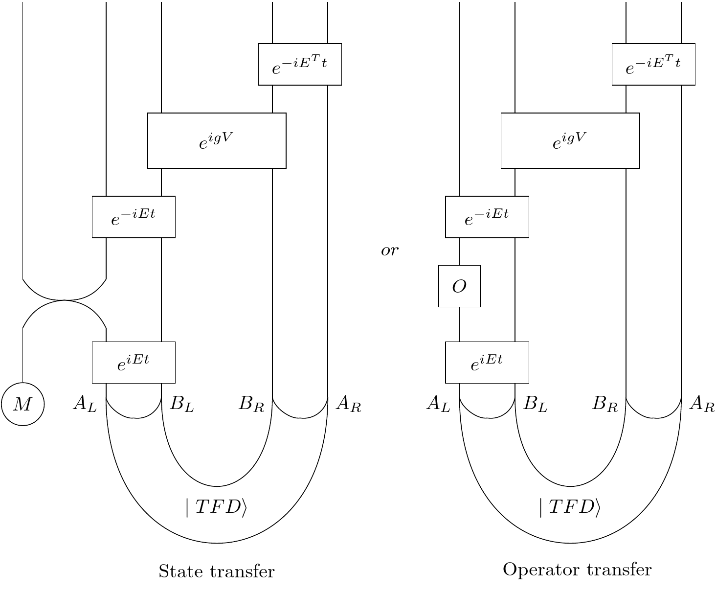
In our first example, we choose a random Hamiltonian and implement the state transfer protocol. We start with a message initialized to $ \begin{pmatrix} 1 \\ 0 \end{pmatrix} $, swap it into the left black hole, and then evolve. We then consider the expectation value of the Z operator on the corresponding qubit on the right side. Because of the tranpose, this should be -1 if all goes well (as opposed to +1). We still need a g value: a strength of the V coupling. So we try different g's to see what works and graph the expectation value of the Z operator against the value of g.
# RANDOM HAMILTONIAN MODEL
%matplotlib notebook
import matplotlib.pyplot as plt
import qutip as qt
import numpy as np
from qutip.qip.operations import swap

##############################################################

def construct_tfd(E, beta=0):
    El, Ev = E.eigenstates()
    return (1/np.sqrt((-beta*E).expm().tr()))*\
             sum([np.exp(-(1/2)*beta*l)*\
                 qt.tensor(Ev[i].conj(), Ev[i])\
                    for i, l in enumerate(El)])

def construct_coupling(n):
    return\
    (1/(n-1))*sum([qt.tensor(*[qt.sigmaz()\
                       if j == i else qt.identity(2) \
                            for j in range(2*n)])*
                   qt.tensor(*[qt.sigmaz()\
                        if j == i+n else qt.identity(2) \
                            for j in range(2*n)])
                                for i in range(1, n)])

##############################################################

n = 7
beta = 0

IDn = qt.identity(2**n)
IDn.dims = [[2]*n, [2]*n]

E = qt.rand_herm(2**n)
E.dims = IDn.dims
tfd = construct_tfd(E, beta=beta)
tfd.dims = [[2]*(2*n), [1]*(2*n)]

msg = qt.basis(2,0)
state = qt.tensor(msg, tfd)

V = construct_coupling(n)

##############################################################

def worm(g, t, state, E, V, IDn):
    state2 = qt.tensor(qt.identity(2), (1j*E*t).expm(), IDn)*state
    state3 = swap(N=2*n+1, targets=[0,1])*state2
    state4 = qt.tensor(qt.identity(2), (-1j*E*t).expm(), IDn)*state3
    state5 = qt.tensor(qt.identity(2), (1j*g*V).expm())*state4
    state6 = qt.tensor(qt.identity(2), IDn, (-1j*E.trans()*t).expm())*state5
    return qt.expect(qt.sigmaz(), state6.ptrace(n+1))

t = 10
G = np.linspace(-10, 25, 40)
Z = [worm(g, t, state, E, V, IDn) for g in G]

best_g = G[np.argmin(np.array(Z))]
print(best_g)

plt.plot(G, Z, linewidth=2.0)
plt.show()
In our second example, we use a specific Hamiltonian--actually two!: the kicked Ising model. Its time evolution can be described in two parts:
$$ U = U_{K}U_{I} $$$$ U_{K} = e^{ib \sum_{i} X_{i}} $$$$ U_{I} = e^{iJ\sum_{i} Z_{i}Z_{i+1} + i \sum_{i} h_{i}Z_{i}} $$The model parameters are $J, b, $ and $h_{i}$. It turns out that if $ J = b = \frac{\pi}{4} $ and the $ h_{i} $ drawn uniformly from a Gaussian distribution, then the model is "maximally chaotic" if you look at how the entanglement entropy of subsystems grows (if you start with a product state). The first term is the kick, the second term is the Ising.
Otherwise, the same as before. Compare the produced plot with that included in arXiv:1911.06314.
# KICKED ISING MODEL
%matplotlib notebook
import matplotlib.pyplot as plt
import qutip as qt
import numpy as np
from qutip.qip.operations import swap

##############################################################

def construct_tfd(E, beta=0):
    El, Ev = E.eigenstates()
    return (1/np.sqrt((-beta*E).expm().tr()))*\
             sum([np.exp(-(1/2)*beta*l)*\
                 qt.tensor(Ev[i].conj(), Ev[i])\
                    for i, l in enumerate(El)])

def construct_coupling(n):
    return\
    (1/(n-1))*sum([qt.tensor(*[qt.sigmaz()\
                       if j == i else qt.identity(2) \
                            for j in range(2*n)])*
                   qt.tensor(*[qt.sigmaz()\
                        if j == i+n else qt.identity(2) \
                            for j in range(2*n)])
                                for i in range(1, n)])

##############################################################

n = 7
beta = 0

IDn = qt.identity(2**n)
IDn.dims = [[2]*n, [2]*n]

##############################################################

J = b = np.pi/4
h = np.random.normal(scale=0.5, size=n)
HK = b*sum([\
        qt.tensor(*[qt.sigmax()\
            if i == j else qt.identity(2)\
                for j in range(n)])\
                    for i in range(n)])
HI = J*sum([\
        qt.tensor(*[qt.sigmaz()\
            if j == i else qt.identity(2)\
                for j in range(n)])*\
        qt.tensor(*[qt.sigmaz()\
            if j == i+1 else qt.identity(2)\
                for j in range(n)])
                for i in range(n-1)])+\
       sum([h[i]*\
               qt.tensor(*[qt.sigmaz()\
                   if j == i else qt.identity(2)\
                       for j in range(n)])\
                           for i in range(n)])
UK = (1j*HK).expm()
UI = (1j*HI).expm()
U = UK*UI

##############################################################

E = HI + HK
tfd = construct_tfd(E, beta=beta)
tfd.dims = [[2]*(2*n), [1]*(2*n)]

msg = qt.basis(2,0)
state = qt.tensor(msg, tfd)

V = construct_coupling(n)

##############################################################

def worm(g, t, state, E, V, IDn):
    state2 = qt.tensor(qt.identity(2), U.dag()**t, IDn)*state
    state3 = swap(N=2*n+1, targets=[0,1])*state2
    state4 = qt.tensor(qt.identity(2), U**t, IDn)*state3
    state5 = qt.tensor(qt.identity(2), (1j*g*V).expm())*state4
    state6 = qt.tensor(qt.identity(2), IDn, U.trans()**t)*state5
    return qt.expect(qt.sigmaz(), state6.ptrace(n+1))

t = 10
G = np.linspace(-10, 25, 40)
Z = [worm(g, t, state, E, V, IDn) for g in G]

best_g = G[np.argmin(np.array(Z))]
print(best_g)

plt.plot(G, Z, linewidth=2.0)
plt.show()
It turns out that we can cement the analogy with quantum teleportation. The ZZ coupling is a classical coupling: it's actually diagonal! So we can replace it with a measurement and correction analogously to the teleportation case. We make Z measurements on all the "carrier qubits": in other words, the B qubits on the left side. For each we get an eigenvalue +1 or -1. We then act on the B qubits on the right with:
$$ e^{ig\sum_{i} z_{i}Z_{i}/(a-b)} $$In the above, i ranges over the B qubits on the right, and little z is the obtained eigenvalue. a is the number of A qubits on a side (in this case 1), b is the number of B qubits on a side.
# RANDOM HAMILTONIAN MODEL / MEASUREMENT
%matplotlib notebook
import matplotlib.pyplot as plt
import qutip as qt
import numpy as np
from qutip.qip.operations import swap

##############################################################

def construct_tfd(E, beta=0):
    El, Ev = E.eigenstates()
    return (1/np.sqrt((-beta*E).expm().tr()))*\
             sum([np.exp(-(1/2)*beta*l)*\
                 qt.tensor(Ev[i].conj(), Ev[i])\
                    for i, l in enumerate(El)])

def construct_coupling(n):
    return\
    (1/(n-1))*sum([qt.tensor(*[qt.sigmaz()\
                       if j == i else qt.identity(2) \
                            for j in range(2*n)])*
                   qt.tensor(*[qt.sigmaz()\
                        if j == i+n else qt.identity(2) \
                            for j in range(2*n)])
                                for i in range(1, n)])

def optimize_g(n, t, state, E, V, ID2, IDn):
    def prep_worm(n, t, E, ID2, IDn):
        U1 = qt.tensor(qt.identity(2), (1j*E*t).expm(), IDn)
        U2 = swap(N=2*n+1, targets=[1,2])
        U3 = qt.tensor(qt.identity(2), (-1j*E*t).expm(), IDn)
        U5 = qt.tensor(qt.identity(2), IDn, (-1j*E.trans()*t).expm())
        return [U5, U3*U2*U1]
    def worm(n, g, V, state, ops, ID2):
        A, B = ops
        U4 = qt.tensor(qt.identity(2), (1j*g*V).expm())
        state = A*U4*B*state
        return qt.expect(qt.sigmaz(), state.ptrace(n+1))
    G = np.linspace(0, 15, 60)
    worm_prep = prep_worm(n, t, E, ID2, IDn)
    Z = [worm(n, g, V, state, worm_prep, ID2) for g in G]
    g = G[np.argmin(np.array(Z))]
    return g

##############################################################

n = 4
beta = 0

IDn = qt.identity(2**n)
IDn.dims = [[2]*n, [2]*n]

E = qt.rand_herm(2**n)
E.dims = IDn.dims
tfd = construct_tfd(E, beta=beta)
tfd.dims = [[2]*(2*n), [1]*(2*n)]

msg = qt.basis(2,0)
state = qt.tensor(msg, tfd)
g = optimize_g(n, t, state, E, V, ID2, IDn)

##############################################################

def measure(op, i, state):
    n = len(state.dims[0])
    L, V = op.eigenstates()
    rho = state.ptrace(i)
    probabilities = np.array([(rho*V[j]*V[j].dag()).tr() for j in range(len(V))])
    probabilities = probabilities/sum(probabilities)
    choice = np.random.choice(list(range(len(L))), p=probabilities)
    projector = qt.tensor(*[V[choice]*V[choice].dag()\
                            if j == i else qt.identity(2)\
                                for j in range(n)])
    projector.dims = [state.dims[0], state.dims[0]]
    state = (projector*state).unit()
    return L[choice], state

def worm(n, g, t, state, E, IDn):
    state2 = qt.tensor(qt.identity(2), (1j*E*t).expm(), IDn)*state
    state3 = swap(N=2*n+1, targets=[0,1])*state2
    state4 = qt.tensor(qt.identity(2), (-1j*E*t).expm(), IDn)*state3

    #print("measuring left B qubits in the z-basis...")
    measurements = []
    for i in range(2, n+1):
        l, state4 = measure(qt.sigmaz(), i, state4)
        measurements.append(l)
        #print("got %.2f on qubit %d" % (l, i))
    #print("applying  unitary correction...")
    correction = (1j*g*sum([z*qt.tensor(*[qt.sigmaz()\
                              if j == 2+n+i else qt.identity(2)\
                              for j in range(2*n+1)])/(n-1)\
                                     for i, z in enumerate(measurements)])).expm()
    state5 = (correction*state4).unit()
    state6 = qt.tensor(qt.identity(2), IDn, (-1j*E.trans()*t).expm())*state5
    return qt.expect(qt.sigmaz(), state6.ptrace(n+1))

print(worm(n, g, t, state, E, IDn))
Next, we consider evolving the wormwhole system continously in time, step by step through the state transfer protocol. First we optimize our g value. Then we construct the wormhole, this time using an entangled qubit as a reference. We track the mutual information between the reference qubit and those in the wormhole system instead of the Z expectation values. In a sense, using the entangled qubit trick allows us to defer our choice of which state we actually through into the wormhole. Using the "jump" method, we can project the reference state into some desired state, and see which state comes out the other side.
# TIME STEP RANDOM HAMILTONIAN MODEL
%matplotlib notebook
import matplotlib.pyplot as plt
import qutip as qt
import numpy as np
from qutip.qip.operations import swap

##############################################################

def construct_tfd(E, beta=0):
    El, Ev = E.eigenstates()
    return (1/np.sqrt((-beta*E).expm().tr()))*\
             sum([np.exp(-(1/2)*beta*l)*\
                 qt.tensor(Ev[i].conj(), Ev[i])\
                    for i, l in enumerate(El)])

def construct_coupling(n):
    return\
    (1/(n-1))*sum([qt.tensor(*[qt.sigmaz()\
                       if j == i else qt.identity(2) \
                            for j in range(2*n)])*
                   qt.tensor(*[qt.sigmaz()\
                        if j == i+n else qt.identity(2) \
                            for j in range(2*n)])
                                for i in range(1, n)])

def optimize_g(n, t, state, E, V, ID2, IDn):
    def prep_worm(n, t, E, ID2, IDn):
        U1 = qt.tensor(ID2, (1j*E*t).expm(), IDn)
        U2 = swap(N=2*n+2, targets=[1,2])
        U3 = qt.tensor(ID2, (-1j*E*t).expm(), IDn)
        U5 = qt.tensor(ID2, IDn, (-1j*E.trans()*t).expm())
        return [U5, U3*U2*U1]
    def worm(n, g, V, state, ops, ID2):
        A, B = ops
        U4 = qt.tensor(ID2, (1j*g*V).expm())
        state = A*U4*B*state
        e = qt.entropy_mutual(state.ptrace((0, n+2)), 0, 1)
        #print("g: %.3f e: %.10f" % (g, e))
        return e
    G = np.linspace(0, 15, 60)
    worm_prep = prep_worm(n, t, E, ID2, IDn)
    ents = [worm(n, g, V, state, worm_prep, ID2) for g in G]
    g = G[np.argmax(np.array(ents))]
    return g

##############################################################

dt = 0.05
t = 10
n = 4
beta = 0

ID2 = qt.identity(4)
ID2.dims = [[2,2], [2,2]]
IDn = qt.identity(2**n)
IDn.dims = [[2]*n, [2]*n]

E = qt.rand_herm(2**n)
E.dims = IDn.dims
tfd = construct_tfd(E, beta=beta)
tfd.dims = [[2]*(2*n), [1]*(2*n)]

ref_msg = qt.bell_state("00")
state = qt.tensor(ref_msg, tfd)

V = construct_coupling(n)
g = optimize_g(n, t, state, E, V, ID2, IDn)

##############################################################

entropies = [qt.entropy_mutual(\
                state.ptrace((0, i)), 0, 1)\
                     for i in range(1, 2*n+2)]
entropies = entropies[:1+n] + entropies[1+n:][::-1]

##############################################################

fig, ax = plt.subplots()
ax.set_ylabel('entanglement')
plt.ylim([0,0.5])
plt.xticks(np.arange(2*n+1), ["O"]+\
                   ["L%d" % (i) for i in range(n)]+\
                   ["R%d" % (i) for i in range(n, 0, -1)])
bar = ax.bar(list(range(2*n+1)), entropies)

##############################################################

def update(n, state, fig, bar):
    entropies = [qt.entropy_mutual(\
                    state.ptrace((0, i)), 0, 1)\
                        for i in range(1, 2*n+2)]
    entropies = entropies[:1+n] + entropies[1+n:][::-1]
    for b, e in zip(bar, entropies):
        b.set_height(e)
    fig.canvas.draw()
    plt.pause(0.00001)

##############################################################

state = qt.tensor(ref_msg, tfd)

print("evolving left back in time...")
U1 = qt.tensor(ID2, (1j*E*dt).expm(), IDn)
for i in range(int(t/dt)):
    state = U1*state
    update(n, state, fig, bar)

print("swapping in msg...")
state = swap(N=2*n+2, targets=[1,2])*state

print("evolving left forward in time...")
U2 = qt.tensor(ID2, (-1j*E*dt).expm(), IDn)
for i in range(int(t/dt)):
    state = U2*state
    update(n, state, fig, bar)

print("coupling...")
U3 = qt.tensor(ID2, (1j*V*dt).expm())
for i in range(int(g/dt)):
    state = U3*state
    update(n, state, fig, bar)

print("evolving right forward in time")
U4 = qt.tensor(ID2, IDn, (-1j*E.trans()*dt).expm())
for i in range(int(t/dt)):
    state = U4*state
    update(n, state, fig, bar)

print("done!")

def jump(n, guy, state):
    proj = qt.tensor(guy*guy.dag(), *[qt.identity(2) for i in range(2*n+1)])
    return (proj*state).unit().ptrace(n+2)

guy = qt.basis(2,0)
guy2 = jump(n, guy, state)
print("in:")
print(guy)
print("out:")
print(guy2)
Finally, we consider evolving the whole system continuously in time without steps, just under the following hamiltonian:
$$ \eta = E_{L} + E_{R}^{T} - gV $$$$ H = \eta - \langle TFD \mid \eta \mid TFD \rangle $$The point of the expectation value is that the TFD should be an approximate ground state of E.
# CONTINUOUS TIME RANDOM HAMILTONIAN MODEL
%matplotlib notebook
import matplotlib.pyplot as plt
import qutip as qt
import numpy as np
from qutip.qip.operations import swap

##############################################################

def construct_tfd(E, beta=0):
    El, Ev = E.eigenstates()
    return (1/np.sqrt((-beta*E).expm().tr()))*\
             sum([np.exp(-(1/2)*beta*l)*\
                 qt.tensor(Ev[i].conj(), Ev[i])\
                    for i, l in enumerate(El)])

def construct_coupling(n):
    return\
    (1/(n-1))*sum([qt.tensor(*[qt.sigmaz()\
                       if j == i else qt.identity(2) \
                            for j in range(2*n)])*
                   qt.tensor(*[qt.sigmaz()\
                        if j == i+n else qt.identity(2) \
                            for j in range(2*n)])
                                for i in range(1, n)])

def optimize_g(n, t, state, E, V, ID2, IDn):
    def prep_worm(n, t, E, ID2, IDn):
        U1 = qt.tensor(ID2, (1j*E*t).expm(), IDn)
        U2 = swap(N=2*n+2, targets=[1,2])
        U3 = qt.tensor(ID2, (-1j*E*t).expm(), IDn)
        U5 = qt.tensor(ID2, IDn, (-1j*E.trans()*t).expm())
        return [U5, U3*U2*U1]
    def worm(n, g, V, state, ops, ID2):
        A, B = ops
        U4 = qt.tensor(ID2, (1j*g*V).expm())
        state = A*U4*B*state
        e = qt.entropy_mutual(state.ptrace((0, n+2)), 0, 1)
        #print("g: %.3f e: %.10f" % (g, e))
        return e
    G = np.linspace(0, 15, 60)
    worm_prep = prep_worm(n, t, E, ID2, IDn)
    ents = [worm(n, g, V, state, worm_prep, ID2) for g in G]
    g = G[np.argmax(np.array(ents))]
    return g

##############################################################

dt = 0.05
t = 10
n = 4
beta = 0

ID2 = qt.identity(4)
ID2.dims = [[2,2], [2,2]]
IDn = qt.identity(2**n)
IDn.dims = [[2]*n, [2]*n]

E = qt.rand_herm(2**n)
E.dims = IDn.dims
tfd = construct_tfd(E, beta=beta)
tfd.dims = [[2]*(2*n), [1]*(2*n)]

ref_msg = qt.bell_state("00")
state = qt.tensor(ref_msg, tfd)

V = construct_coupling(n)
g = optimize_g(n, t, state, E, V, ID2, IDn)

ETA = qt.tensor(E, IDn) + qt.tensor(IDn, E) - g*V
H = ETA - qt.expect(ETA, tfd)
U = qt.tensor(ID2, (-1j*H*dt).expm())

##############################################################

entropies = [qt.entropy_mutual(\
                state.ptrace((0, i)), 0, 1)\
                     for i in range(1, 2*n+2)]
entropies = entropies[:1+n] + entropies[1+n:][::-1]

##############################################################

fig, ax = plt.subplots()
ax.set_ylabel('entanglement')
plt.ylim([0,0.5])
plt.xticks(np.arange(2*n+1), ["O"]+\
                   ["L%d" % (i) for i in range(n)]+\
                   ["R%d" % (i) for i in range(n, 0, -1)])
bar = ax.bar(list(range(2*n+1)), entropies)

##############################################################

def update(n, state, fig, bar):
    entropies = [qt.entropy_mutual(\
                    state.ptrace((0, i)), 0, 1)\
                        for i in range(1, 2*n+2)]
    entropies = entropies[:1+n] + entropies[1+n:][::-1]
    for b, e in zip(bar, entropies):
        b.set_height(e)
    fig.canvas.draw()
    plt.pause(0.00001)

##############################################################

state = qt.tensor(ref_msg, tfd)
state = swap(N=2*n+2, targets=[1,2])*state

for i in range(1000):
    state = U*state
    update(n, state, fig, bar)