Consider a bunch of qubits evolving under some random unitary operator. If we wanted to run this on a quantum computer, for example, we'd want to compile down that unitary into a series of, say, one and two qubit operators that we apply in a sequence since these are simpler to implement. Consider a single qubit in our group, which starts off separable from the rest. As time goes on, maybe it interacts with another qubit: then, generically, the two qubits will get entangled. Each of those qubits then goes off and gets entangled with more qubits, and now it's possible all four are entangled. And so on. In other words, entanglement spreads between quantum systems like an epidemic.
Here's an easy way to get a handle on this. Below is a python implementation of above: a bunch of qubits start of separable, and we evolve them under some randomly selected time evolution. We want to track how one qubit gets entangled with the rest. One easy way to do this is to instead start off with a maximally entangled pair of qubits. One stays outside the group, the other one evolves with the rest of the group. We can then calculate the entanglement between the one who stays outside and all the ones in the group in turn, and track it over time. Think of it like we have two qubits connected by Ariadne's thread; we toss one in and it gets scrambled into the rest, but we can keep track of it by following the thread home.
What's a good measure of entanglement though? A classical measure is the quantum mutual information:
$$ QMI(A, B) = S(A) + S(B) - S(A, B)$$$$ S = - tr( \rho \ ln \rho ) = - \sum_{\lambda} \lambda \ ln \lambda $$$S$ is called the Von Neumann entropy. In the latter part the sum is over eigenvalues $ \lambda $ of $ \rho $.
%matplotlib notebook
import matplotlib.pyplot as plt
import numpy as np
import qutip as qt

n = 4
dt = 0.01
t_max = 1000

ref, rest = qt.bell_state("00"), qt.tensor(*[qt.rand_ket(2) for i in range(n)])
state = qt.tensor(ref, rest)
state.dims = [[2]*(n+2), [1]*(n+2)]

E = qt.rand_herm(2**(n+1))
U = qt.tensor(qt.identity(2), (-1j*dt*E).expm())
U.dims = [[2]*(n+2), [2]*(n+2)]

entropies = [qt.entropy_mutual((state*state.dag()).ptrace((0, i)), 0, 1) for i in range(1, n+2)]

fig, ax = plt.subplots()
ax.set_xlabel('qubit')
ax.set_ylabel('entanglement')

bar = ax.bar(list(range(1, n+2)), entropies)

for i in range(t_max):
    state = U*state
    entropies = [qt.entropy_mutual((state*state.dag()).ptrace((0, i)), 0, 1) for i in range(1, n+2)]
    for b, e in zip(bar, entropies):
        b.set_height(e)
    fig.canvas.draw()
    plt.pause(0.0001)
Just like we can track a qubit as it gets scrambled among the rest, we could also keep track of an operator, watch how it starts off localized and then gets spread out over the whole Hilbert space.
So we're interested in tracking in some sense the size/complexity of the operator $ O(t) = e^{iEt} O e^{-iEt} $ as it evolves in time.
Now just as quantum states form a vector space, operators also form a vector space. For example, I can write any 2x2 Hermitian matrix in the following 4-vector form:
$$ H = tI + xX + yY + zZ $$So given an operator H I can expand it in terms of a real (t, x, y, z) vector. One way to do this is to use the generalization of the inner product for matrices: $ (tr(H), tr(X^{\dagger}H), tr(Y^{\dagger}H), tr(Z^{\dagger}H)) $. But we know another way: We could multiply I, X, Y, Z and H all by the cup state and then take the normal inner product: $ ( \langle I\cup \mid H \cup \rangle , \langle X \cup \mid H \cup \rangle , \langle Y \cup \mid H \cup \rangle , \langle Z \cup \mid H \cup \rangle ) $.
I could decompose a 2x2 unitary in the same way: the components would then be generally complex. Cool, but does the same work for the nxn case? Yes, there's always some basis for Hermitian matrices. But we want to consider spaces of qubits and it turns out that the following 16 operators forms a basis for two qubit operators:
$$ \begin{matrix}II & IX & IY & IZ \\ XI & XX & XY & XZ \\ YI & YX & YY & YZ \\ ZI & ZX & ZY & ZZ\end{matrix} $$And then same goes for the n-qubit case: we take all arrangements of the Pauli operators, and we can expand any operator in the so-called Pauli basis. The point is that in the Pauli basis we can define the notion of the size of an operator. For the 1 qubit case, $I$ has size 0, while $X, Y, Z$ each have size 1. In the 2 qubit case, we have 1 operator of size 0, 6 operators of size 1, and 9 operators of size 2. We'll write $ |P| $ for the size of a Pauli operator P.
So we have the idea that generically operators grow in size over time. Let's watch it happen.
%matplotlib notebook
import matplotlib.pyplot as plt
import qutip as qt
import numpy as np
from itertools import product

def pauli_basis(n):
    IXYZ = {"I": qt.identity(2), "X": qt.sigmax(), "Y": qt.sigmay(), "Z": qt.sigmaz()}
    names, ops = [], []
    for P in product(IXYZ, repeat=n):
        names.append("".join(P))
        ops.append(qt.tensor(*[IXYZ[p] for p in P]))
    return names, ops

def to_pauli(op, Pops):
    return np.array([(o.dag()*op).tr() for o in Pops])/np.sqrt(len(Pops))

n = 2
dt = 0.01
Pnames, Pops = pauli_basis(n)

H = qt.rand_herm(2**n)
H.dims = [[2]*n, [2]*n]
U = (-1j*dt*H).expm()
O = qt.tensor(*[qt.sigmax() if i == 0 else qt.identity(2) for i in range(n)])

probabilities = [(a*a.conj()).real for a in to_pauli(O, Pops)]

fig, ax = plt.subplots()
ax.set_xlabel('paulis')
ax.set_ylabel('probabilities')
plt.xticks(np.arange(len(Pnames)), Pnames)
bar = ax.bar(list(range(len(Pnames))), probabilities)

t_max = 5000
for i in range(t_max):
    O = U.dag()*O*U
    probabilities = [(a*a.conj()).real for a in to_pauli(O, Pops)]
    for b, p in zip(bar, probabilities):
        b.set_height(p)
    fig.canvas.draw()
    plt.pause(0.0001)
In fact, we could think about the operator as a quantum particle undergoing its own Schrodinger evolution but defined on a graph where nodes are Pauli matrices and node are connected by edges when they are one operator different from another.
So now we can put some interesting facts together. We know that:
$$ O_{L} (-t) \mid TFD \rangle \to \rho_{\beta, R}^{\frac{1}{2}} O_{R}^{T} (t) \mid \cup \rangle $$$$ O_{R}^{T} (t) \mid TFD \rangle \to O_{R}^{T} (t) \rho_{\beta, R}^{\frac{1}{2}} \mid \cup \rangle $$And our general setup is:
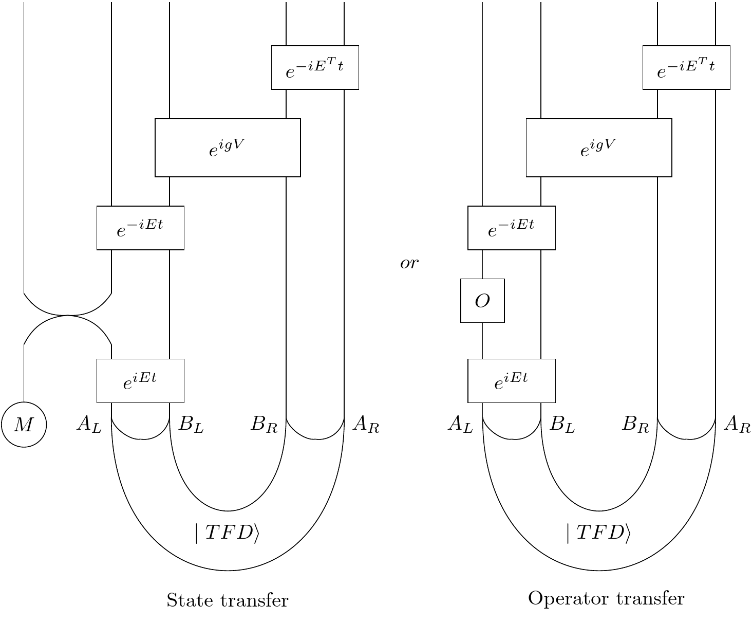
The question is what properties does our \(E)\ have to have for this to work? In the state transfer picture, we throw a qubit in on the left in the past, which then should get completely scrambled over the whole left side. To the extend that the qubit is scrambled over the whole thing, we could say that the qubit is "deeper inside" the black hole. Then our coupling should somehow transfer our deep qubit from the left to the right, and then the forward time evolution on the right side should unscramble it and Bob's your uncle.
Following arXiv:1911.06314, it turns out that energy operators that have the right scrambling properties exhibit something called "perfect size winding." And even if the size winding isn't perfect, you can still often get stuff through.
The authors of the aforementioned paper provide the following ansatz:
$$ \big( \rho_{\beta, R}^{\frac{1}{2}} O_{R}^{T} (t) \big)(t) = \sum_{Paulis} e^{i \alpha \frac{|P|}{n}}r_{p}P $$Here the sum is over all the n-qubit Paulis where n is the number of qubits on the right side! Since we can see that this is an operator that only acts on the right. $r_{p}$ is some real coefficient, $P$ is the given Pauli, and $ \alpha $ is some overall phase. (Incidentally, in the limit of large size for a random P, $ \alpha = \frac{4}{3}g$--we'll come back to the $g$.) We can see that in the Pauli basis, each Pauli basis vector has a phase proportional to its size. In other words, for perfect sizing winding Hamiltonians, in the Pauli basis, the phases wind around at a speed proportional to its size.
Considering that $ \big( \rho_{\beta, R}^{\frac{1}{2}} O_{R}^{T} (t) \big)^{\dagger} = O_{R}^{T} (t) \rho_{\beta, R}^{\frac{1}{2}} $, we can say:
$$ O_{L} (-t) \mid TFD \rangle = \sum_{Paulis} e^{i \alpha \frac{|P|}{n}}r_{p}\mid P \rangle$$$$ O_{R}^{T} (t) \mid TFD \rangle = \sum_{Paulis} e^{-i \alpha \frac{|P|}{n}}r_{p}\mid P \rangle$$Which is of course:
$$ O_{L} (-t) \mid TFD \rangle = \sum_{Paulis} e^{i \alpha \frac{|P|}{n}}r_{p}P_{L}\mid \cup \rangle$$$$ O_{R}^{T} (t) \mid TFD \rangle = \sum_{Paulis} e^{-i \alpha \frac{|P|}{n}}r_{p}P_{L}\mid \cup \rangle$$The only difference between $ O_{L} (-t) $ and $ O_{R}^{T} (t) $ is the direction of the winding, whether clockwise or counterclockwise.
Recall our choice of V operator from before.
$$ V = \frac{1}{b-a} \sum_{i}^{b} Z_{i, L} Z_{b-i, R} $$Its role is simply to unwind the phases. It turns out that the ZZ coupling is sensitive enough to size to do the job.
Finally, when $ \beta = 0 $, in other words, at infinite temperature when the TFD reduces down to the $\cup $, $ \rho_{\beta, R}^{\frac{1}{2}} O_{R}^{T} $ is Hermitian and has real expansion coefficients in the Pauli basis. And so no unwinding is necessary!