Consider the Schrodinger equation.
$$ \dot \psi = -iE\psi$$The dot above the $\psi$ means the change in time of $\psi$, in other words, its first derivative. $\psi$ is our state vector. $ E $ is the energy operator: $ \langle \psi \mid E \mid \psi \rangle $ is the expected value of the energy. One of the most important equations in linear algebra is the one relating the "eigenvalues" and "eigenvectors" of an operator.
$$ E\mid v \rangle = \lambda\mid v \rangle$$The action of an operator E on an eigenvector $ v $ is just $ v $ multiplied by a scalar $ \lambda $. "Eigen" in German means "the same." So the eigenvectors of an operator are the vectors which are left "unrotated" by the operator: the eigenvectors are merely scaled by some eigenvalue. Now the eigenvalues can be complex, leading to a complex rotation, or phase shift, but the vector itself isn't rotated as a whole. And if the eigenvalue is 0, then the eigenvector remains completely unchanged. Now, operators corresponding to "observables" in quantum mechanics are Hermitian: in otherwords, they are equal to their conjugate transpose. $ H = H^{\dagger} $: these matrices have real eigenvalues, so their expectation values are real; and their eigenvectors are all orthogonal, and so they form a complete basis for the space on which they operate.
So what is the Schrodinger equation saying? It's saying according to quantum mechanics, the time derivative of an energy eigenstate is just given by the state itself times $-1j\lambda$. And if $ \lambda = 0 $, the state doesn't change at all. So we describe change in quantum mechanics in terms of those states which don't change in time. To wit, if you're in an energy eigenstate, you stay in an energy eigenstate, just phasing around at a certain rate given by the eigenvalue. Superpositions of energy eigenstates, in other words, states with an uncertainty about their energy, correspond to states that change in time.
There are many ways to approach solving the Schrodinger equation depending on the circumstances. Let's work through just one example.
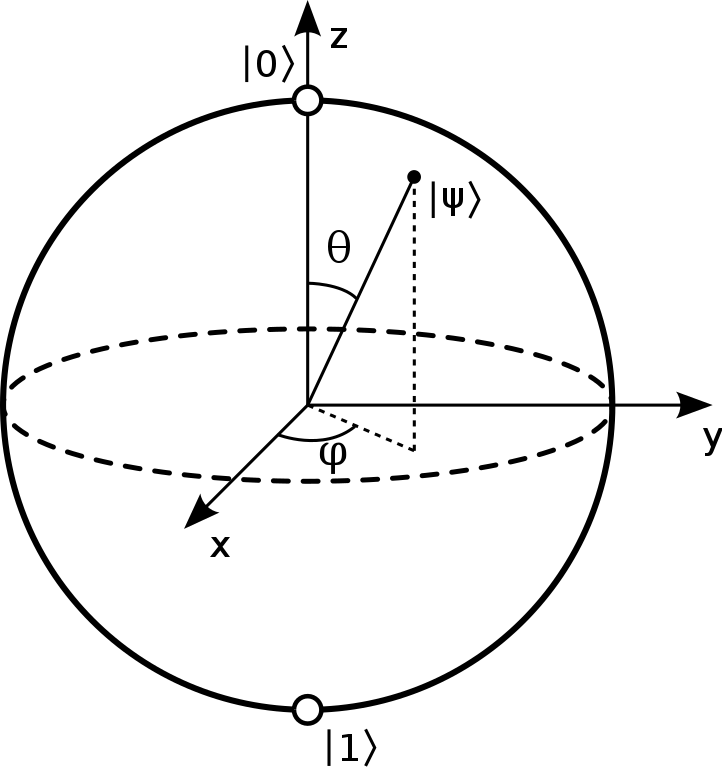
But first, a quick detour into the geometry of a qubit so we can interpret our results. The qubit is a little spinning object. It can be described in terms of its axis of rotation (which gives a point on the sphere) along with a phase which describes how it's turned around that axis. The axis of rotation can be easily obtained:
$$ (x, y, z) = (\langle \psi \mid X \mid \psi \rangle, \langle \psi \mid Y \mid \psi \rangle, \langle \psi \mid Z \mid \psi \rangle)$$It's just the "expected value" of the Pauli X, Y, Z operators. Remember we can't observe this axis of rotation directly: if we measure X, Y, or Z, we are projecting into an eigenstate with some probability, thus destroying whatever the origional rotation axis was. Another point is that for a pure state, the (x, y, z) point lies on the surface of the sphere, while for mixed/partial states it lies within the sphere. For the perfectly mixed state (given by, for example, the partial state of the left or right half of a cup), we find (0, 0, 0): there's complete ambiguity about which axis the qubit is spinning around.
We note that the eigenstates of X, which are orthogonal complex vectors, correspond to X+ and X-, antipodal points on the sphere. The same goes for Y and Z.
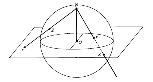
A geometric way of interpreting the relationship between a qubit and its rotation axis can be given in terms of the stereographic projection. First, we recognize that our qubit is a complex projective space which means there's a map from a qubit to $ \left\{ \mathbb{C} + \infty \right\} $.
$ \begin{pmatrix} a \\ b \end{pmatrix} \to \frac{a}{b} $ if $b \neq 0 $ else $ \infty $
Inversely:
$ c \to \begin{pmatrix} c \\ 1 \end{pmatrix} $ if $c \neq \infty$ else $\begin{pmatrix} 1 \\ 0 \end{pmatrix} $
We can normalize the qubit if we like. It's clear that the qubit encodes its axis up to multiplication by a scalar. (And that projective spaces allow you to divide by 0!)
We then do an inverse stereographic projection from $ \left\{ \mathbb{C} + \infty \right\} $ to the 2-sphere. By choosing a "north pole," we are choosing an axis of quantization. The usualy choice is in terms of eigenstates of Z.
$ x+iy \to (\frac{2x}{1 + x^{2} + y^{2}}, \frac{2y}{1 + x^{2} + y^{2}}, \frac{-1 + x^{2} + y^{2}}{1 + x^{2} + y^{2}}) $ or $ (0, 0, 1) $ if $ \infty $
Inversely: $ (x, y, z) \to \frac{x}{1-z} + i\frac{y}{1-z} $ or $ \infty $ if $ z = 1 $
So here's a problem. Suppose we start at the north pole $ \begin{pmatrix} 1 \\ 0 \end{pmatrix} $ and we want to rotate around the X axis. Solving the Schrodinger equation will allow us to watch this unfold in time. We take our energy operator to be X.
$$ \dot \psi = -iX\psi $$Now let's expand this out, taking into account that our state vector is two dimensional. We'll use x and y to denote these components although that may be confusing.
$$ \begin{pmatrix} \dot x \\ \dot y \end{pmatrix} = -i\begin{pmatrix} 0 & 1 \\ 1 & 0 \end{pmatrix}\begin{pmatrix} x \\ y \end{pmatrix} $$$$ \begin{pmatrix} \dot x \\ \dot y \end{pmatrix} = \begin{pmatrix} 0 & -i \\ -i & 0 \end{pmatrix}\begin{pmatrix} x \\ y \end{pmatrix} $$$$ \begin{pmatrix} \dot x \\ \dot y \end{pmatrix} = \begin{pmatrix} -iy \\ -ix \end{pmatrix} $$$$ \frac{dx}{dt} = -iy \\ \frac{dy}{dt} = -ix $$There's a standard way to solve such equations. First, we have to find the eigenvalues and eigenvectors of the matrix $ \begin{pmatrix} 0 & -i \\ -i & 0 \end{pmatrix} $, which we'll call A.
We recall our equation relating eigenvalues and eigenvectors $ A\mid v \rangle = \lambda\mid v \rangle $:
$$ A\mid v \rangle = \lambda\mid v \rangle $$$$ A\mid v \rangle - \lambda\mid v \rangle = 0 $$$$ (A - \lambda I)\mid v \rangle = 0 $$In the above, 0 is the 0 vector. If the last equation is true, it means that the matrix $ (A - \lambda I) $ is not invertible: after all, it sends all the eigenvectors of A to the zero vector from which there is no return. It's a linear algebraic fact that this implies that the determinant of $ (A - \lambda I) $ is 0.
Recall that the determinant of a 2x2 matrix is: $ \begin{vmatrix} a & b \\ c & d \end{vmatrix} = ad - bc $.
$$ \begin{vmatrix} 0 - \lambda & -i \\ -i & 0-\lambda \end{vmatrix} = 0$$So we have eigenvalues $ \pm i $. (This makes sense: the X operator has eigenvalues $ \pm 1 $.
According to our equation,
$$ \begin{pmatrix} - \lambda & -i \\ -i & -\lambda \end{pmatrix} \begin{pmatrix} v_{0} \\ v_{1} \end{pmatrix} = \begin{pmatrix} 0 \\ 0 \end{pmatrix} $$So we plug in $ \lambda = i $.
$$ \begin{pmatrix} -i & -i \\ -i & -i \end{pmatrix} \begin{pmatrix} v_{0} \\ v_{1} \end{pmatrix} = \begin{pmatrix} 0 \\ 0 \end{pmatrix} $$So we could take $ \lambda = i , v = \begin{pmatrix} 1 \\ -1 \end{pmatrix} $, although any scalar multiple would do. Then we do the same for $ \lambda = -1 $.
$$ \begin{pmatrix} i & -i \\ -i & i \end{pmatrix} \begin{pmatrix} v_{0} \\ v_{1} \end{pmatrix} = \begin{pmatrix} 0 \\ 0 \end{pmatrix} $$$$ i v_{0} -i v_{1} = 0 $$$$ v_{0} = v_{1} $$So we can take $ \lambda = -i , v = \begin{pmatrix} 1 \\ 1 \end{pmatrix} $. (Indeed, these are also the eigenvalues of the X operator itself.)
We can immediately write down a general solution to our original equation.
$$ \begin{pmatrix} x(t) \\ y(t) \end{pmatrix} = c_{0} e^{it} \begin{pmatrix} 1 \\ -1 \end{pmatrix} + c_{1} e^{-it} \begin{pmatrix} 1 \\ 1 \end{pmatrix} $$The exponentials are $ e^{\lambda t} $, and $ c_{0} $ and $ c_{1} $ are coefficients which are undetermined. We can determine them by choosing an initial condition, that at time t = 0, we start at the north pole: $ \begin{pmatrix} 1 \\ 0 \end{pmatrix} $.
Our matrix equation then reduces to:
$$ \begin{pmatrix} 1 \\ 0 \end{pmatrix} = c_{0} e^{i0} \begin{pmatrix} 1 \\ -1 \end{pmatrix} + c_{1} e^{-i0} \begin{pmatrix} 1 \\ 1 \end{pmatrix} = \begin{pmatrix} c_{0} \\ - c_{0} \end{pmatrix} + \begin{pmatrix} c_{1} \\ c_{1} \end{pmatrix} = \begin{pmatrix} c_{0} + c_{1}\\ -c_{0} + c_{1} \end{pmatrix}$$$$ c_{0} + c_{1} = 1 $$$$ -c_{0} + c_{1} = 0 $$$$ c_{0} = c_{1} $$$$ 2c_{1} = 1 $$$$ c_{0}, c_{1} = \frac{1}{2}$$So our final solution is:
$$ \begin{pmatrix} x(t) \\ y(t) \end{pmatrix} = \frac{1}{2} \Big( e^{it} \begin{pmatrix} 1 \\ -1 \end{pmatrix} + e^{-it} \begin{pmatrix} 1 \\ 1 \end{pmatrix} \Big) $$$$ \begin{pmatrix} x(t) \\ y(t) \end{pmatrix} = \frac{1}{2} \begin{pmatrix} e^{it} + e^{-it} \\ e^{-it} - e^{it} \end{pmatrix} $$# Let's check it in python.
import qutip as qt
import numpy as np
import vpython as vp
scene = vp.canvas(background=vp.color.white)
def xyz(qubit):
return [qt.expect(qt.sigmax(), qubit),\
qt.expect(qt.sigmay(), qubit),\
qt.expect(qt.sigmaz(), qubit)]
qubit = lambda t: (1/2)*qt.Qobj(np.array([np.exp(1j*t) + np.exp(-1j*t),\
np.exp(-1j*t) - np.exp(1j*t)]))
vp.sphere(color=vp.color.blue, opacity=0.5)
vstar = vp.sphere(pos=vp.vector(*xyz(qubit(0))), radius=0.3, emissive=True)
dt, t, t_max = 0.01, 0, 10
while t < t_max:
vstar.pos = vp.vector(*xyz(qubit(t)))
t += dt
vp.rate(30)
But there's another way we can calculate the time evolution. We can reformulate the Schrodinger equation ( $\dot \psi = -iE\psi )$ as:
$$ \psi (t) = e^{-iEt}\psi (0)$$$ e^{-iEt} $ is the matrix exponential. It has many interesting properties. It's a matrix which at t=0 is just the identity matrix. Its columns are solutions to the differential equation we solved before. And it is able to impart time evolution to a quantum state. We generalize the classic Euler formula ($ e^{i\pi} = -1 $) in a big way. In quantum mechanics, if $E $ is hermitian, then $ e^{-iEt} $ is unitary: in other words, it has purely imaginary eigenvalues, and preserves probability. It's these matrices that represent time evolution. Geometrically, in the case of our qubit, we can think of $ e^{-iX\frac{\theta}{2}} $ as a rotation by $ \theta $ degrees around the $ X $ axis.
One way to define the matrix exponential is in terms of an infinite series, just like the normal exponential function.
$$ e^{Et} = I + At + \frac{A^{2}t^{2}}{2!} + \frac{A^{3}t^{3}}{3!} + \frac{A^{4}t^{4}}{4!} + \dots $$The exclaimation point means take the factorial.
We can also define it terms of the general solution we found before. Recall:
$$ \begin{pmatrix} x(t) \\ y(t) \end{pmatrix} = \begin{pmatrix} c_{0} e^{it} \\ -c_{0} e^{it} \end{pmatrix} + \begin{pmatrix} c_{1} e^{-it} \\ c_{1} e^{-it} \end{pmatrix} $$We need the matrix exponential to be the identity matrix $\begin{pmatrix} 1 & 0 \\ 0 & 1 \end{pmatrix} $ at t = 0 and have solutions to the differential equation as columns.
So at t = 0, we require for the first column:
$$ \begin{pmatrix} 1 \\ 0 \end{pmatrix} = \begin{pmatrix} c_{0} \\ -c_{0} \end{pmatrix} + \begin{pmatrix} c_{1} \\ c_{1} \end{pmatrix} $$And so:
$$ 1 = c_{0} + c_{1} $$$$ 0 = -c_{0} + c_{1} $$$$ c_{0} = c_{1} $$$$ 1 = 2c_{0} $$$$ c_{0}, c_{1} = \frac{1}{2} $$So our first column will be $ \frac{1}{2} \begin{pmatrix} e^{it} + e^{-it} \\ e^{-it} - e^{it} \end{pmatrix} $.
At t = 0, we require for the second column:
$$ \begin{pmatrix} 0 \\ 1 \end{pmatrix} = \begin{pmatrix} c_{0} \\ -c_{0} \end{pmatrix} + \begin{pmatrix} c_{1} \\ c_{1} \end{pmatrix} $$And so:
$$ 0 = c_{0} + c_{1} $$$$ 1 = -c_{0} + c_{1} $$$$ c_{0} = -c_{1} $$$$ 1 = -2c_{0} $$$$ c_{0} = -\frac{1}{2}, c_{1} = \frac{1}{2} $$So our second column will be $ \frac{1}{2} \begin{pmatrix} e^{-it} - e^{it} \\ e^{it} + e^{-it} \end{pmatrix} $.
Putting the two together gives us our matrix:
$$ e^{-iEt} = \frac{1}{2} \begin{pmatrix} e^{it} + e^{-it} & e^{-it} - e^{it} \\ e^{-it} - e^{it} & e^{it} + e^{-it} \end{pmatrix} $$# Let's test it out in python
import qutip as qt
import numpy as np
import vpython as vp
scene = vp.canvas(background=vp.color.white)
def xyz(qubit):
return [qt.expect(qt.sigmax(), qubit),\
qt.expect(qt.sigmay(), qubit),\
qt.expect(qt.sigmaz(), qubit)]
initial_qubit = qt.Qobj(np.array([1,0]))
MEXP = lambda t: (1/2)*qt.Qobj(np.array([[np.exp(1j*t)+np.exp(-1j*t), np.exp(-1j*t)-np.exp(1j*t)],\
[np.exp(-1j*t)-np.exp(1j*t), np.exp(1j*t)+np.exp(-1j*t)]]))
vp.sphere(color=vp.color.blue, opacity=0.5)
vstar = vp.sphere(pos=vp.vector(*xyz(qubit(0))), radius=0.3, emissive=True)
dt, t, t_max = 0.01, 0, 10
while t < t_max:
vstar.pos = vp.vector(*xyz(MEXP(t)*initial_qubit))
t += dt
vp.rate(30)
Finally, a third way of calculating the matrix exponential. We can instead diagonalize our matrix. First, we form a change-of-basis matrix: a matrix whose columns are eigenvectors of $-iE$.
$$ P = \begin{pmatrix} 1 & 1 \\ -1 & 1 \end{pmatrix} $$If we multiply the change-of-basis matrix by a vector, it gives the vector in the reference frame defined by the original matrix. Operators can be transformed too, but they require action on two sides. So we define the inverse of the change-of-basis matrix. This is easy in the 2x2 case.
$$ A^{-1} = \begin{pmatrix} a & b \\ c & d \end{pmatrix}^{-1} = \frac{1}{det A}\begin{pmatrix} d & -b \\ -c & a \end{pmatrix} $$$$ P^{-1} = \frac{1}{2}\begin{pmatrix} 1 & -1 \\ 1 & 1 \end{pmatrix} $$We then consider:
$$ P^{-1} A P = \frac{1}{2}\begin{pmatrix} 1 & -1 \\ 1 & 1 \end{pmatrix} \begin{pmatrix} 0 & -i \\ -i & 0 \end{pmatrix} \begin{pmatrix} 1 & 1 \\ -1 & 1 \end{pmatrix} = \frac{1}{2}\begin{pmatrix} 1 & -1 \\ 1 & 1 \end{pmatrix}\begin{pmatrix} i & -i \\ -i & -i \end{pmatrix} = \frac{1}{2}\begin{pmatrix} 2i & 0 \\ 0 & -2i \end{pmatrix} = \begin{pmatrix} i & 0 \\ 0 & -i \end{pmatrix}$$In its "own" basis, the matrix A is a diagonal matrix with its eigenvalues along the diagonal. In this basis, the matrix exponential is actually just the naive:
$$ e^{\begin{pmatrix} i & 0 \\ 0 & -i \end{pmatrix}t} = \begin{pmatrix} e^{it} & 0 \\ 0 & e^{-it} \end{pmatrix} $$Then we transform back home.
$$ P D P^{-1} = \begin{pmatrix} 1 & 1 \\ -1 & 1 \end{pmatrix}\begin{pmatrix} e^{it} & 0 \\ 0 & e^{-it} \end{pmatrix}\frac{1}{2}\begin{pmatrix} 1 & -1 \\ 1 & 1 \end{pmatrix} = \frac{1}{2}\begin{pmatrix} 1 & 1 \\ -1 & 1 \end{pmatrix} \begin{pmatrix} e^{it} & - e^{it} \\ e^{-it} & e^{-it} \end{pmatrix} = \frac{1}{2}\begin{pmatrix} e^{it} + e^{-it} & e^{-it} - e^{it} \\ e^{-it} - e^{it} & e^{-it} + e^{it} \end{pmatrix} $$This is precisely what we got before.
# In practice...
import qutip as qt
import numpy as np
import vpython as vp
scene = vp.canvas(background=vp.color.white)

def xyz(qubit):
    return [qt.expect(qt.sigmax(), qubit),\
            qt.expect(qt.sigmay(), qubit),\
            qt.expect(qt.sigmaz(), qubit)]

dt = 0.01
qubit = qt.Qobj(np.array([1,0]))
U = (-1j*qt.sigmax()*dt).expm()

vp.sphere(color=vp.color.blue, opacity=0.5)
vstar = vp.sphere(pos=vp.vector(*xyz(qubit)), radius=0.3, emissive=True)

for i in range(5000):
    qubit = U*qubit
    vstar.pos = vp.vector(*xyz(qubit))
    vp.rate(30)
It's interesting that a vector transforms under a change-of-basis like $P\mid v \rangle $, but an operator transforms like $P^{-1} A P $. It turns out we can actually formulate time evolution in quantum mechanics in two different but completely equivalent ways.
The first is the Schrodinger picture. We have $ \mid \psi (t) \rangle = e^{-iEt}\mid \psi (0) $, and we can track the expectation values of interesting operators on the time evolving state: $ \langle \psi (t) \mid O_{0} \mid \psi (t) \rangle, \langle \psi (t) \mid O_{2} \mid \psi (t) \rangle \dots $, but the operators are fixed for all time as a reference.
The second is the Heisenberg picture. Here the state is fixed once and for all, and it's the operators that evolve in time. It's the difference between rotating a point on a sphere, and rotating the X/Y/Z axes so that the point appears to rotate in exactly the same way.
So we have $ \mid \psi (t) \rangle $ fixed, but operators evolve like:
$$ O(t) = e^{iEt} O e^{-iEt} $$It is a nice fact about unitary matrices that their conjugate transpose is their inverse! Given a hermitian matrix $E$:
$$ U^{\dagger} = U^{-1} = (e^{-iEt})^{\dagger} = e^{iEt} $$So all the operators evolve like $ \langle \psi \mid O_{0}(t) \mid \psi \rangle, \langle \psi \mid O_{2}(t) \mid \psi \rangle \dots $