Introduction to Finite Frames and RIC-POVM's
Maturing out of our reflexive habit of working with orthonormal bases, we can instead work with an overcomplete basis or "frame," which can have as many elements as we like. In fact, with probability 1, any randomly chosen set of vectors ($n \ge d$) will form a frame.
Let's just think about $d=2$ real vector space. Why not a frame made of 5 vectors?
import numpy as np
import scipy as sc
import scipy.linalg
np.set_printoptions(precision=4, suppress=True)

d, n = 2, 5
R = np.random.randn(d, n); R
We can form the Gram matrix, aka the matrix of inner products:
G = R.T @ R; G
One condition for everything being kosher is that the Gram matrix ought to be rank-$d$.
np.round(np.linalg.svd(G)[1], decimals=4)
We should also check out:
R @ R.T
We'll have a frame if the latter has non-0 determinant aka is full rank. This means that the rows of $R$ are linearly independent.
np.linalg.det(R @ R.T)
By the way, the technical definition of a frame is a set of vectors $\{v\}$, for which there are constants $a, b > 0$ such that for any vector $u$:
$$ a ||u||^2 \leq \sum_{i} |\langle u|v_{i}\rangle|^2 \leq b||u||^2 $$The $a$ and $b$ are called frame bounds, and this definition is always satisfied if the aforementioned conditions are true. We won't be using this definition too much.
Analysis and Synthesis
Suppose we have some 2D point:
point = np.random.randn(2); point
We can expand it in terms of our frame vectors:
c = R.T @ point; c
R.T is often called the "analysis" operator.
How do we recover the original point, though?
We use the dual frame, obtained by taking the pseudo-inverse of R.
The inner products with the frame vectors turn out to be the weights on the dual basis vectors, which via summation recover the original point.
D = np.linalg.pinv(R); D
sum([c[i]*D[i] for i in range(n)])
Or:
D.T @ c
D.T is often called the "synthesis" operator.
It works because:
D.T @ R.T
Conversely, we could have expanded in the dual basis:
c = D @ point; c
R @ c
Another way of thinking about this "recovery" procedure: instead, we could take the pseudo-inverse of the Gram matrix.
Ginv = np.linalg.pinv(G); Ginv
If we have our frame coordinates:
c = R.T @ point; c
Acting with $G^{-1}$ will give us the coordinates in the dual basis:
Ginv @ c
So that:
R @ Ginv @ c
In other words, using $G^{-1}$, we can avoid explicitly invoking the dual basis.
Tight Frames
We might consider restrictions on our frames. Different kinds of frames are useful for different purposes.
For example, everyone loves tight frames. We can get one via a generalization of a polar decomposition for rectangular matrices. Starting with a random $d \times n$ matrix $R$, we decompose as $R = UH$, where the rows of $U$ are orthonormal, and $H$ is Hermitian. Then we throw out the $H$ part.
R = np.random.randn(d, n)
R = sc.linalg.polar(R)[0]; R
R.T @ R
The point is that:
R @ R.T
So the frame is the same as its dual! In other words, the analysis operator is R.T and the synthesis operator is R.
point
c = R.T @ point; c
R @ c
More generally, any frame for which $R R^{\dagger}$ is proportional to the identity is a "tight frame," so that the dual frame is proportional to the original frame. In terms of the "frame bounds" from before, a tight frame means that $a=b$. And when $a=b=1$, this is known as a "Parseval frame."
Also, for a tight frame, the Gram matrix is a rank-$d$ projector.
np.linalg.eig(R.T @ R)[0]
Unit Norm Tight Frames
We might also be interested not just in tight frames, but in "unit norm tight frames". As the name suggests, each vector has unit norm.
One easy way to get one is to alternate between "tightening" and "normalizing" our vectors until we're satisfied.
def random_funtf(d, n, rtol=1e-15, atol=1e-15):
    R = np.random.randn(d, n)
    done = False
    while not (np.allclose(R @ R.T, (n/d)*np.eye(d), rtol=rtol, atol=atol) and\
               np.allclose(np.linalg.norm(R, axis=0), np.ones(n), rtol=rtol, atol=atol)):
        R = sc.linalg.polar(R)[0]
        R = np.array([state/np.linalg.norm(state) for state in R.T]).T
    return R
R = random_funtf(2, 5); R
R.T @ R
R @ R.T
Notice that we've had to demand $RR^{\dagger}$ to be $\frac{n}{d} I$.
point
c = R.T @ point; c
(d/n)*R @ c
Equiangular Frames
As I say, there are many kinds of frames that people are interested in, which have various geometric and/or information theoretic properties.
One of the classics of the genre are the so-called "equiangular frames," which are made up of vectors which form equal angles with each other (or more properly, the absolute values of the inner products are all the same).
These are great for many reasons, not least because they provide very resilient representations of data even if you should lose a few components.
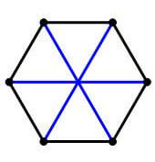
There are, however, geometrical restrictions on the maximum number of equiangular lines you can have in a given dimension. For example, in $d=2$, you can have a maximum of $3$ equiangular lines.
The $3$ are easy to construct:
R = np.array([[r.real, r.imag] for r in [np.exp(2j*np.pi*i/3) for i in range(3)]]).T; R
R.T @ R
R @ R.T
The 3 lines form the diagonals of a hexagon.
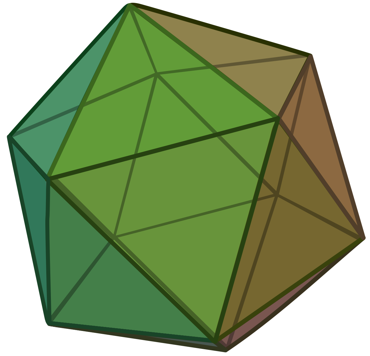
In three dimensions, an equiangular frame is provided by the icosahedron, which has 20 faces and 12 vertices: its six diagonals provide the frame vectors.
def circular_shifts(v):
    """
    Returns all shifted versions of a vector, e.g.:
        [1,2,3]
        [3,1,2]
        [2,3,1]
    """
    shifts = [v]
    for i in range(len(v)-1):
        u = shifts[-1][:]
        u.insert(0, u.pop())
        shifts.append(u)
    return shifts

def icosahedron_frame():
    """
    Returns equiangular frame based on the icosahedron in three dimensions.
    """
    phi = (1+np.sqrt(5))/2 # golden ratio
    # 12 vertices provided by circular shifts of the four vectors
    vertices = [np.array(v) for v in
                   circular_shifts([0, 1, phi]) + \
                   circular_shifts([0, -1, -phi]) + \
                   circular_shifts([0, 1, -phi]) + \
                   circular_shifts([0, -1, phi])]
    # throw out the antipodal vectors
    keep = []
    for i, a in enumerate(vertices):
        for j, b in enumerate(vertices):
            if i != j and np.allclose(a, -b) and j not in keep:
                keep.append(i)
    # normalize
    return np.array([e/np.linalg.norm(e) for i, e in enumerate(vertices) if i in keep]).T
R = icosahedron_frame(); R
R.T @ R
R @ R.T
Check out frame_viz.py to play around with different kinds of 2D frames!
You'll be able to drag around a point in 2D. Press c to show standard Cartesian axes, and the projections of the point onto them. Press f to show the frame vectors and the projections onto them. Press d to show the dual vectors and the projections onto them. Press q to show the reconstruction of the point by a weighted sum of frame vectors (provided by the inner products with the dual vectors). Press p to show the reconstruction of the point by a weighted sum of dual vectors (provided by the inner products with the frame vectors).
Note that to get the projections right, we need to divide frame (dual) coordinates by the norm squared of the corresponding frame (dual) vectors.
Because:
R = np.random.randn(2, 3); R
point
If we want to project the point onto the three frame vectors, we can use the projectors formed from the outer products $rr^{T}$, where $r$ is unit norm. This amounts to dividing by $||r||^2$.
np.array([np.outer(r/np.linalg.norm(r), r/np.linalg.norm(r))@point for r in R.T])
Meanwhile, we have our inner products:
c = R.T @ point; c
To recover the projections, we multiply each of the inner products by the vector, divided by the norm squared.
np.array([c[i]*R.T[i]/np.linalg.norm(R.T[i])**2 for i in range(3)])
Finally, in the case of 2D, we have another way of visualizing things. Press 3 to check it out.
We can interpret the three inner products with the frame vectors as a point in 3D.
c
Moreover, D will be a $3 \times 2$ matrix: we can interpret its 2 columns as specifying two vectors in 3D.
D = np.linalg.pinv(R); D
We can project our 3D point onto these two vectors:
[np.outer(D.T[i], D.T[i])/np.linalg.norm(D.T[i])**2 @ c for i in range(2)]
But this is just the same as weighting each of the two vectors by the Cartesian coordinates of the original point!
[point[i]*D.T[i]/np.linalg.norm(D.T[i])**2 for i in range(2)]
In other words, the three inner products with the frame vector specify a point in 3D. The dual basis specifies two linearly independent axes in 3D. The projection of the 3D point onto these two axes gives two coordinates: these are proportional to the original 2D point in Cartesian coordinates.
RIC-POVM's
Now consider that $3$ is also the dimension of the space of $2 \times 2$ symmetric matrices.
Indeed, we might be interested in this fact if we wanted to do real vector space quantum mechanics.
In real quantum mechanics, pure states are given by 2D vectors $\mid \psi \rangle = \begin{pmatrix}x \\ y \end{pmatrix}$ such that $x^2 + y^2 = 1$, aka points on the circle; or better yet: rank-1 density matrices: $\mid \psi \rangle \langle \psi \mid = \begin{pmatrix}x^2 & xy \\ xy & y^2 \end{pmatrix}$.
More generally, a density matrix might be a higher rank statistical mixture. Any symmetric, positive semi-definite matrix with unit trace will do.
Now here's the big reveal: it turns out that tight frames are just rank-1 POVM's in disguise.
Recall that a POVM, or positive operator valued measure, is a set of positive semi-definite matrices that sum to the identity: $\sum_{i} E_{i} = I$. Each "element" represents an outcome to a generalized quantum measurement that concretely involves entangling your quantum system to an apparatus (with a dimensionality equal to the number of POVM elements) and doing a standard (Von Neumann) measurement on the latter. In the case of a rank-1 POVM, the outcome states of the original sytem will correspond to the normalized POVM elements.
A POVM can have any number of elements (well, I suppose at least two!): but we're interested in "informationally complete" POVM's, which have as many elements as the dimensions of the relevant operator space, aka the space of density matrices, which for real vector space is $\frac{d(d+1)}{2}$. (In complex quantum mechanics, we use not symmetric matrices, but Hermitian matrices, which have $d^2$ parameters.)
If we have enough elements to span the operator space, then the vector of probabilities for each outcome suffice to completely determine the quantum state. And so, among other things, we can do quantum tomography, treating pure states and mixed states on an equal footing, by repeating one measurement over and over again on many copies of a system, instead of having to do different, complementary measurements.
We can upgrade a tight frame into a rank-1 POVM by taking the outer products of the vectors with themselves. (And by the way, it's not at all necessary that POVM elements be rank-1: those we'll be considering here, however, will be.) The POVM condition, as you can see, is satisfied since $RR^{\dagger}$ amounts to $\sum_{i} |r\rangle\langle r|$.
d, n = 2, 3
R = sc.linalg.polar(np.random.randn(d, n))[0]
R @ R.T
E = [np.outer(r, r) for r in R.T]
sum(E)
Given a random density matrix:
def rand_dm(d, n=2):
    # n controls the degree of mixedness
    A = np.random.randn(d, n)
    rho = A @ A.T
    return rho/rho.trace()

rho = rand_dm(2); rho
We can expand it in terms of POVM elements:
p = np.array([(e @ rho).trace() for e in E]); p
sum(p)
The components sum to 1: they are the probabilities for the outcomes to this experiment.
Now how do we get the density matrix back? The dual basis, of course! But how do we find it?
Given a matrix $A$, denote by $|A\rangle \rangle$ the vector you get by reshaping the matrix into a vector.
(If you want to be fancy, you can think of this like $\sum_{i} (A \otimes I)\mid i \rangle\mid i \rangle$, or as $A$ acting on the left on the maximally entangled "cup" state on the doubled Hilbert space, $H_{d} \otimes H_{d}$).
Then form the "(operator) frame operator":
$F = \sum_{i} \mid E_{i} \rangle \rangle \langle \langle E_{i} \mid = \sum_{i} E_{i} \otimes E_{i}$.
I should note that the right hand side is only true if we have rank-1 POVM elements. In that case:
$$ |E_{i}\rangle\rangle = (E_{i} \otimes I) \sum_{j} |j\rangle | j \rangle = (|r_{i}\rangle\langle r_{i}| \otimes I) \sum_{j} |j\rangle | j \rangle = \sum_{j} |r_{i}\rangle\langle r_{i}|j\rangle | j \rangle = |r_{i}\rangle \sum_{j} \langle r_{i} | j \rangle | j \rangle = |r_{i}\rangle |r_{i}\rangle$$So that:
$$ \sum_{i} |E_{i}\rangle\rangle \langle \langle E_{i} | = \sum_{i} |r_{i}\rangle |r_{i}\rangle \langle r_{i} | \langle r_{i} | = \sum_{i} |r_{i}\rangle \langle r_{i}| \otimes | r_{i} \rangle \langle r_{i} | = \sum_{i} E_{i} \otimes E_{i}$$In the second line, we use the fact that $| a \rangle | b \rangle \langle c | \langle d| = |a\rangle\langle c| \otimes |b\rangle\langle d|$.
Finally, take the (pseudo) inverse of $F$. Then, $F^{-1}\mid E_{i}\rangle \rangle = \mid \tilde{E}_{i} \rangle \rangle$, where $\tilde{E}$ is the dual basis.
F = sum([np.kron(e, e) for e in E])
Finv = np.linalg.pinv(F)
D = [(Finv @ e.reshape(d**2)).reshape(d,d) for e in E]
Then, we can recover the original density matrix by weighting the elements of the dual basis by the probabilities and summing:
rho
sum([p[i]*D[i] for i in range(n)])
Conversely, we could expand in dual elements:
q = np.array([(e @ rho).trace() for e in D]); q
And recover the original density matrix by weighting POVM elements and summing
sum([q[i]*E[i] for i in range(n)])
By the way, the dual basis of an informationally complete POVM doesn't form a POVM itself. Indeed, its elements must be indefinite!
Alternatively, instead of working with the dual basis directly, we could play a similar trick from before.
Instead of taking $G^{-1}$, now we take $(G \circ G )^{-1}$ where $\circ$ is the Hadamard (element-wise) square. Instead of expanding in the dual basis, we can act with $(G \circ G )^{-1}$ on the vector of probabilities to get the proper weights for POVM elements required to recover $\rho$.
rho
p
G = R.T @ R
Gsq_inv = np.linalg.inv(G**2)
q = Gsq_inv @ p; q
We can now get our density matrix back:
sum([q[i]*E[i] for i in range(n)])
But we can do a little bit more, which will prove useful.
We could form a matrix of conditional probabilities supposing we repeat our POVM twice. In other words, a matrix of conditional probabilities:
$$ Pr(E_{i}|E_{j}) = tr(E_{i}\frac{E_{j}}{tr(E_{j})})$$After the first measurement, we end up in some $\frac{E_{j}}{tr(E_{j})}$, and then we look at the probabilities that we get some $E_{i}$.
E_given_E = np.array([[(E[i]@(E[j]/E[j].trace())).trace() for j in range(n)] for i in range(n)]); E_given_E
Notice that this related to $(G \circ G )$, except for the fact that we divide by $tr(E_{j})$.
We can take its inverse to obtain the "Born matrix" $\Phi$:
phi = np.linalg.inv(E_given_E); phi
What's the point? If we take our density matrix:
rho
And its probabilities:
p
Then we can form:
q = phi @ p; q
sum(q)
This is nice, because by acting on our vector of probabilities with $\Phi$, we get back a vector of quasi-probabilities: while the components might be negative, they nevertheless sum to 1. And this will prove to be useful.
We can then get our density matrix back by summing over normalized elements of our POVM, weighted by the quasi-probabilities.
sum([q[i]*E[i]/E[i].trace() for i in range(n)])
Moreover, we can also obtain this matrix $\Phi$ from the dual elements. Actually, it's nicer to renormalize the dual elements first so that they have the same weights as the POVM elements.
D = [E[i].trace()*D[i] for i in range(n)]
sum(D)
D_given_D = np.array([[(D[i]@(D[j]/D[j].trace())).trace() for j in range(n)] for i in range(n)]); D_given_D
Expanding in renormalized dual elements gives us our quasiprobabilities:
q = np.array([(d @ rho).trace() for d in D]); q
And as before:
sum([q[i]*E[i]/E[i].trace() for i in range(n)])
And symmetrically:
sum([p[i]*D[i]/D[i].trace() for i in range(n)])
Deforming the Law of Total Probability
Okay, but why should we care?
We're going to consider two measurements on our quantum system, $A$ and $B$, where $A$ is an IC-POVM, and $B$ could be a standard Von Neumann measurement or a POVM, doesn't matter. Let's say it's an IC-POVM.
d, n = 2, 3
A = [np.outer(r, r) for r in sc.linalg.polar(np.random.randn(d, n))[0].T]
B = [np.outer(r, r) for r in sc.linalg.polar(np.random.randn(d, n))[0].T]
rho
We can of course nail down our quantum state by its probabilities on measurement $A$.
p_A = np.array([(a @ rho).trace() for a in A]); p_A
Now we're going to compare two sequences of events.
First: we measure $A$, and then measure $B$. Before we look at the outcome for $A$, however, what probabilities should we assign to the outcomes of $B$?
To figure this out, we could use a matrix of conditional probabilities:
B_given_A = np.array([[(b@a/a.trace()).trace() for a in A] for b in B]); B_given_A
These are the conditional probabilities for each of $B$'s outcomes, given each outcome state of $A$. This gives us conditional probabilities $Pr(B_{i}|A_{j})$.
We end up with a column stochastic matrix:
np.sum(B_given_A, axis=0)
We can then use the law of total probability: $Pr(B_{i}) = \sum_{j} Pr(B_{i}|A_{j}) Pr(A_{j})$.
p_AB = B_given_A @ p_A; p_AB
sum(p_AB)
We can check this. After the measurement of $A$, we should regard our system's state as a statistical mixture of $A$'s outcomes, weighted by the probability of their occurance:
rho_post_A = sum([p_A[i]*a/a.trace() for i, a in enumerate(A)]); rho_post_A
We can then get the $B$ probabilities for this density matrix by taking inner products with $B$'s elements.
p_AB2 = np.array([(b @ rho_post_A).trace() for b in B]); p_AB2
sum(p_AB2)
We get the same probabilities.
To recap: we did measurement of $A$, but didn't look at the answer. We just wanted the probabilities for the future measurement $B$. So we used the law of total probability: $p(B_{i}) = \sum_{j} p(B_{i}|A_{j}) p(A_{j})$.
Okay.
The second experiment is that we leave $A$ hypothetical, but instead just do the $B$ measurement. We know what the answer should be: we just expand in terms of $B$.
p_B = np.array([(b @ rho).trace() for b in B]); p_B
But since our probabilities on $A$ completely nail down the state, there ought to be a way of getting these latter probabilities in terms of them...
It's easy! We simply form the "Born matrix" $\Phi$ from before:
phi = np.linalg.inv([[(a1 @ a0/a0.trace()).trace() for a0 in A] for a1 in A])
And instead of doing:
B_given_A @ p_A
We do:
B_given_A @ phi @ p_A
Hence the name the "Born matrix": it allows us to recover the Born rule. Notice how everything is still formulated in terms of a) the conditional probability matrix for B's outcomes given A's outcomes, and b) the probability vector for A's outcomes.
One can now see the usefulness of:
q = phi @ p_A; q
sum(q)
The fact that $\Phi$ takes us to quasiprobabilities makes sure we play nicely with the conditional probability matrix.
Another way of thinking about this is to form a "conditional quasiprobability matrix":
$$ Qr(B_{i}|\tilde{A}_{j}) = tr(B_{i}\frac{\tilde{A}_{j}}{tr(\tilde{A}_{j})})$$FA = sum([np.outer(e.reshape(d**2), e.reshape(d**2)) for e in A])
FAinv = np.linalg.pinv(FA)
DA = [e.trace()*(FAinv @ e.reshape(d**2)).reshape(d,d) for e in A]
B_given_DA = np.array([[(B[i]@(DA[j]/DA[j].trace())).trace() for j in range(n)] for i in range(n)]); B_given_DA
Then:
B_given_DA @ p_A
Indeed:
np.allclose(B_given_DA, B_given_A@phi)
Perhaps more concretely:
If we perform POVM $A$, then:
$$ \rho \rightarrow \rho^{\prime} = \sum_{i} Pr(A_{i}|\rho)\frac{A_{i}}{tr(A_{i})}$$If we don't perform POVM $A$, then:
$$ \rho \rightarrow \sum_{i} Pr(A_{i}|\rho)\frac{\tilde{A}_{i}}{tr(\tilde{A}_{i})}$$Which is just $\rho$!
If we perform POVM $A$, and then POVM $B$:
$$ \rho \rightarrow \sum_{i} \Big{(} \sum_{j} Pr(B_{i}|A_{j}) Pr(A_{j}|\rho) \Big{)} \frac{B_{i}}{tr(B_{i})} = \sum_{i} Pr(B_{i}|\rho^{\prime}) \frac{B_{i}}{tr(B_{i})}$$If we don't perform POVM $A$, and then do perform POVM $B$:
$$ \rho \rightarrow \sum_{i} \big{(} \sum_{j} Qr(B_{i}|\tilde{A}_{j}) Pr(A_{j}|\rho) \big{)} \frac{B_{i}}{tr(B_{i})} = \sum_{i} Pr(B_{i}|\rho) \frac{B_{i}}{tr(B_{i})} $$And if we did neither:
$$ \rho \rightarrow \sum_{i} \big{(} \sum_{j} Qr(B_{i}|\tilde{A}_{j}) Pr(A_{j}|\rho) \big{)} \frac{\tilde{B}_{i}}{tr(\tilde{B}_{i})} = \sum_{i} Pr(B_{i}|\rho) \frac{\tilde{B}_{i}}{tr(\tilde{B}_{i})} $$Which is just $\rho$!
Quantumness
So in the first case, we did $A$, and afterwards we described our system as a mixed state of A's outcomes, weighted by the probability of them happening. No "coherence" between outcomes: there's just "classical ignorance." And we used the old school law of total probability to get the probabilities for the outcomes of $B$.
In the second case, we didn't do $A$: and so "quantum coherence" was preserved. But we could still get the probabilities for a $B$ measurement from the probabilities of the (hypothetical) $A$ measurement.
One way of thinking of this is that quantum mechanics encourages us to modify the law of total probability. Classically speaking, we could use the law of total probability whether or not we did an intermediate measurement of $A$ before $B$. But quantum mechanically, it matters. If we don't do $A$, we have to stick the Born matrix $\Phi$ in between the conditional probability matrix and the probability vector. In matrix notation, instead of $\vec{Pr(B_{i})} = \hat{Pr(B_{i}|A_{j})}\vec{Pr(A_{j})}$, we have $\vec{Pr(B_{i})} = \hat{Pr(B_{i}|A_{j})}\hat{\Phi}\vec{Pr(A_{j})}$.
Now, if $\Phi$ were the identity, then there would be no difference, as it were, between classical and quantum. No coherence, everything having "objective properties," law of total probability always valid, etc. The lesson of quantum mechanics is that: $\Phi$ is not the identity.
So you might wonder: what measurements are associated with a $\Phi$ such that $\Phi$ is as close to the identity as possible?
With this in mind, we form a quantity we'll call "quantumness": $Q = ||\Phi - I||$.
def quantumness(E):
    phi = np.linalg.inv([[(e1@e0/e0.trace()).trace() for e0 in E] for e1 in E])
    return np.linalg.norm(phi - np.eye(len(E)))
quantumness(A), quantumness(B)
This quantity diagnoses the extent to which the law of total probability is deformed.
Now it's known that SIC-POVM's aka "symmetrically informationally complete POVM's," which correspond to equiangular lines, minimize quantumness. And in fact, the proof that they do so doesn't depend on the particulars of which norm you choose to measure the difference between $\Phi$ and the identity.
In other words, and it makes sense, SIC-POVM's, whose elements all make the same angle with each other, have $\Phi$ matrices as close to the identity as possible. They are the quantum measurements that are "irreducibly quantum."
Now much of the study of SIC-POVM's takes place in the context of real quantum mechanics, I mean, complex vector space quantum mechanics. In this case, SIC-POVM's would correspond to complex equiangular lines, which are a bit more difficult to visualize. And to span the space of density matrices, you'd need $d^2$ of them for dimension $d$.
For example, in the case of $d=2$, the four elements of a SIC-POVM make up the vertices of a regular tetrahedron on the Bloch sphere.
It's been conjectured, and widely believed, on the basis of a great deal of theoretical and computational effort, that SIC-POVM's exist in all complex dimensions. And conditional on this being true, then we know the irreducibly quantum measurements in any dimension: they are the SIC's.
Here's the thing, though.
As I've said: in real quantum mechanics, RIC-POVM's (real informationally complete POVM's) require $n=\frac{d(d+1)}{2}$ elements. As we've seen, this is fine for $d=2$: in this case, $n=3$, and we have the "Mercedes-Benz" frame. So too, all is well in $d=3$. Then $n=6$, and we have our icosahedron.
But then the shit hits the fan.
Here's a table listing the known maximum number of equiangular lines in different real dimensions compared to the dimensionality of the symmetric operator space.
I've starred the ones where SIC-POVM's can exist, namely: 2, 3, 7, 23 (so far as we know).
| d | max | n |
|---|---|---|
| 2 | 3 | 3* |
| 3 | 6 | 6* |
| 4 | 6 | 10 |
| 5 | 10 | 15 |
| 6 | 16 | 21 |
| 7 | 28 | 28* |
| 8 | 28 | 36 |
| 9 | 28 | 45 |
| 10 | 28 | 55 |
| 11 | 28 | 66 |
| 12 | 28 | 78 |
| 13 | 28 | 91 |
| 14 | 28 | 105 |
| 15 | 36 | 120 |
| 16 | 40 | 136 |
| 17 | 48-49 | 153 |
| 18 | 56-60 | 171 |
| 19 | 72-74 | 190 |
| 20 | 90-94 | 210 |
| 21 | 126 | 231 |
| 22 | 176 | 253 |
| 23 | 276 | 276* |
(Incidentally, the famous Gerzon bound says there definitely can't be more that $\frac{d(d+1)}{2}$ equiangular lines in $\mathbb{R}^n$).
You might wonder: given that (unlike in the complex case), we definitely know there aren't SIC's in all real dimensions, what's the next best thing? Specifically, what are the RIC's with lowest quantumness in each real dimension where a SIC doesn't exist?
It's an open question!